Aspro2 Documentation
![]()

ASPRO 2 User Manual
Date: Apr 4th 2024
Authors:
- Laurent BOURGES — JMMC / OSUG
- Gilles DUVERT — JMMC / IPAG
- Guillaume MELLA — JMMC/ OSUG
[!NOTE] Documentation updates in progress
Release history:
Show previous revisions:
Here are the complete release notes.
Table of contents
- ASPRO 2 User Manual
- Table of contents
- Description
- Supported interferometers and instruments
- Main functionalities
- Requirements
- How to get and run ASPRO 2 ?
- Acknowledgement
- Guided tour
- Interoperability
- ASPRO 2 - Command Line Interface
- Support and change requests
- Sample files
Description
This document will give general information on the new version of ASPRO named "ASPRO 2" to constitute the "ASPRO 2 User Manual".
ASPRO 2 is a Java standalone program that helps you to prepare observations on various optical interferometers.
Supported interferometers and instruments
- VLTI (Period 84 - 116)
- MIDI (2T) until Period 94
- AMBER (3T) until Period 101
- PIONIER (4T) starting from Period 86
- GRAVITY (4T) starting from Period 98, (GRAVITY_FT to check the fringe tracker ability to track faint or unresolved targets)
- MATISSE (4T) starting from Period 103, (MATISSE_LM & MATISSE_N to describe the internal L/M & N instruments)
- Supported Adaptive Optics:
- UTs: MACAO until Period 114, GPAO since Period 114
- ATs: NAOMI
- VLTI (Future Period) for experimental instruments
- GRAVITY (4T) with more configurations (relocation)
- MATISSE (4T) with more configurations (relocation)
- CHARA
- CLASSIC (2T)
- CLIMB (3T)
- MIRCX (4T, 5T, 6T) + MYSTIC (K)
- PAVO (2T, 3T)
- SPICA (6T)
- Former instruments:
- FRIEND (2T, 3T)
- JOUFLU (2T)
- MIRC (4T, 5T, 6T)
- VEGA (2T, 3T, 4T)
- SUSI
- PAVO (2T)
- NPOI (preliminary / out-dated support)
- CLASSIC (4T)
- VISION (4T, 5T, 6T)
- DEMO (demo interferometer and instruments for VLTI schools)
Xml configuration files are provided as the ASPRO 2 Configuration package and evolve with releases.
Public ASPRO 2 configuration description is available:
Please give us your feedback if you want another interferometer or instrument to be supported or if you find mistakes in the configuration. We are trying to maintain the configuration as exact as possible, but it is really difficult to have the correct & up-to-date information about instruments ...
[!NOTE]
- ASPRO 2 started by Java Web Start always uses the latest ASPRO 2 Configuration package (automatic updates require an internet connection).
- If you download and launch the Aspro2.jar file, please upgrade when a new release is proposed to get the latest ASPRO 2 software & ASPRO 2 Configuration package.
- Please use the
Helpmenu /Configuration Release notesaction to see release notes of the ASPRO 2 Configuration package in use.
Main functionalities
- Dynamic User Interface: any change made on GUI widgets is taken into account on plots immediately
- Load / Save an observation file: allows the user to save his work at any moment. The xml file produced can be reopened later (for off-line use, for example), and is convenient to save all information relative to a list of targets, which can be sent to collaborators, observers at the interferometer, etc...
- Interferometer sketch: display baselines of the selected configuration(s)
- Observability plot: represents time intervals when the source can be observed with transit and elevation marks, night and twilight zones, delay line compensation for the selected baselines, (best) PoPs (CHARA), telescope shadowing (VLTI) and zenithal restriction, pointing restrictions due to the moon avoidance and the wind direction
- UV Coverage plot: shows projected baselines on the UV plan and an image of the source model to see the UV coverage of the source
- OIFits viewer: provides several OIFits data plots (square visibility and closure phase vs spatial frequency ...) including error bars and spectral dispersion
- Multi configuration support to have an overview of UV coverages of one source observed with different configurations
- Target editor: show complete target information, edit missing target magnitudes and associate calibrators to your science targets
- Model editor: each source can have its own object model composed of several elementary models (punct, disk, ring, gaussian, limb darkened disk ...) or an user-defined model (FITS image)
- Interoperability using SAMP (VO protocol):
- Import targets from VO tools like Simbad, VizieR, Topcat using VOTable format (version 1.1 and 1.2)
- SearchCal to search calibrators for your science target(s)
- LITpro to prepare your model fitting using generated OIFits file(s) and the object model of your current target
- OIFits Explorer or OImaging to prepare your data processing
- A2P2 to submit your Observing Blocks directly into ESO P2 tool
- Observing Blocks can be generated:
- for VLTI instruments to be imported in the ESO P2 tool (OBX import) (deprecated)
- for the CHARA VEGA instrument using the Star list format (deprecated)
- OIFits file generation with error and noise modelling
- OIFitsExplorer and OImaging integration to plot your simulated observation data and perform image reconstructions
- Export (/Print): every plot can be exported as either a PNG image or a PDF document. Of course the PDF output is better as it uses vector based graphics and any PDF reader can print it correctly: no "Print" action available, please print the PDF document using your favorite PDF viewer!
- Standard JMMC actions: feedback report, news, release notes and FAQ
Requirements
- Java Runtime Environment (JRE) 8 or newer: Java 11 or 17 or 21 (OpenJDK LTS release) is recommended (security fixes + Long Term Support)
- any PDF reader to display and print any exported plot
- An Internet connection to resolve star identifiers using the CDS Simbad service and get past observation logs
[!NOTE]
- Java 6 or 7 is no more supported by JMMC applications, so Java 8 or newer is recommended.
- Java 21 is supported but only (OpenJDK 17 + IcedTeaWeb 1.8) do provide the Java Web Start support.
OpenJDK binary packages are available through several providers:
- Eclipse Adoptium OpenJDK builds: https://adoptium.net/
- Azul Zulu builds: https://www.azul.com/downloads/zulu-community/
- Liberica OpenJDK: https://bell-sw.com/pages/downloads/
JavaWebStart (IcedTeaWeb) binary packages are available through several providers:
- AdoptOpenJDK IcedTeaWeb builds: https://adoptopenjdk.net/icedtea-web.html
- Azul free IcedTeaWeb builds: https://www.azul.com/downloads/icedtea-web-community/
- OpenWebStart installers (Windows / Mac OS / Linux): https://openwebstart.com/download/
How to get and run ASPRO 2 ?
The easiest way consists in using the JMMC AppLauncher application which is able to run JMMC applications (Aspro 2, SearchCal, LITpro) and other VO tools when needed (relying on Java Web Start to start applications).
An internet connection is required to use Java Web Start and get the latest release: ASPRO 2.
Of course, both Java Web Start and ASPRO 2 support offline mode i.e. ASPRO 2 can work without any internet connection.
Once downloaded, you should have a shortcut icon "Aspro 2" on your desktop:
![]()
Alternatively you can start it again later using the Java Web Start Viewer and click on "Aspro 2":
javaws -viewer
If Java Web Start is not working properly on your environment or if ASPRO 2 needs more memory (1024m by default), you can download the ASPRO 2 (JAR file) and run ASPRO 2 using the following command:
java -Xms1024m -Xmx4096m -jar Aspro2-Version.jar
where:
- Xms: gives the minimum heap memory size (1024 mb = 1 gb)
- Xmx: gives the maximum heap memory size (4096 mb = 4 gb)
[!NOTE] Look at the memory monitor in the status bar to know how much memory is available (depending on the loaded user models) and potentially clean up memory (garbage collection) by clicking on the memory's progress bar.
Look at the JMMC Tools page and the Release page to see the complete list of JMMC tools with related links to news, release notes and FAQs...
[!NOTE] You can run multiple instances of ASPRO 2 at the same time, but it may be confusing when you want to use interoperability with other applications: take care of SAMP's client id reported in the title bar to properly identify the appropriate application instance.
Acknowledgement
If this software was helpful in your research, please add this sentence in the acknowledgement section of your articles, as it will support further development of new tools for interferometry:
    This research has made use of the Jean-Marie Mariotti Center
    \texttt{Aspro2} service \footnote{Available at http://www.jmmc.fr/aspro}.
ASPRO 2 depends on many open source libraries including these important astronomical / VO libraries:
- JSkyCalc Observability constraints and sky display based on JSkyCalc by J. R. Thorstensen, Dartmouth College
- nom.tam.fits The Java FITS library (nom.tam.fits) has been developed which provides efficient I/O for FITS images and binary tables. Made by Dr Thomas A. McGlynn, HEASARC
- JSAMP JSAMP is a Java toolkit for use with the Simple Applications Messaging Protocol. Made by Mark Taylor, Bristol University
The exhaustive list of open source libraries is available: view credits
Guided tour
How to run a simple preparation scenario ?
- Launch ASPRO 2
- Set the main observation settings (interferometer, instrument, configuration ...) and constraints (date ...)
- Enter your observation targets using the the Simbad star resolver
- Navigate among tab panels to see outputs and other options
To complete your observation preparation, you can:
- use the Target Editor to define your object models, edit missing magnitudes and calibrators manually if needed
- or use SearchCal to find calibrators automatically
- export to PDF documents, Observing Blocks or OIFits files ...
Of course you can save your complete observation settings using the File menu / Save action to open it later using the File menu / Open observation action.
Besides the File / Open Recent menu lists up to 10 recent observation settings to quickly open any of them.
[!NOTE]
- On every plot panel, you can use the
Filemenu /Export plot to PDFaction to export it as a PDF document (and print it).- Alternatively you can export the plot as a PNG image by using the plot context menu (right mouse click) and choose the
Save Asaction.- Plots are zoomable using the mouse wheel or making mouse gestures: top left to bottom right to zoom in, right to left to reset the zoom.
Main observation settings
The main panel is always present at the top of the application window to let you define main observation settings:
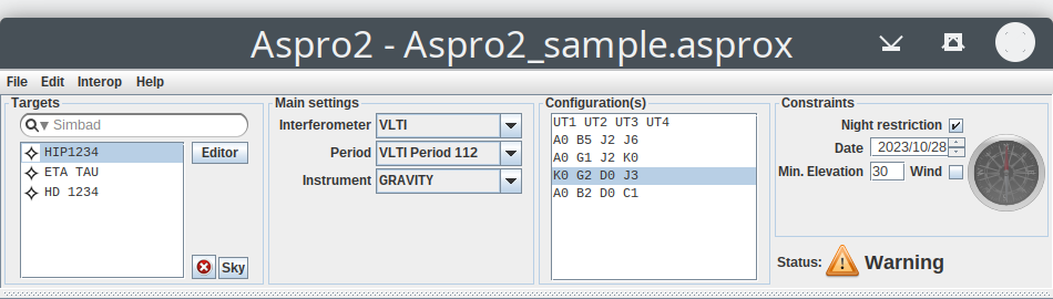
This panel is divided in four parts:
- Targets: add / remove / edit your targets
- Main settings: define main settings (interferometer, instrument ...)
- Configuration(s): select one or more configurations (baselines)
- Constraints: define less important settings (date, night restriction ...)
[!NOTE] Any change made to these fields will be taken into account immediately on plots
Target definition
To add a new target in the target list, the simplest way consist in typing its identifier (name) in the Simbad star resolver and press the Enter key to get its coordinates and other information using the CDS Simbad service.
An error can occur if the target identifier is not present in Simbad or if ASPRO 2 can not access to internet (proxy or firewall problems).
If Simbad returns multiple matches for a given identifier, the following error message is displayed:
Multiple objects found (please refine your query):
'uy': [ NAME UY Aur A, NAME UY Aur B ]
To add multiple targets at once, enter their identifiers separated by ';' (semicolon character) in the star resolver or copy / paste your target list (one identifier per line). Of course, the Simbad query takes more time to proceed then a summary of the query results is displayed.
[!NOTE]
- the Simbad star resolver uses several Simbad mirrors (France, USA and their corresponding fixed IP addresses) automatically if any error occurs. However, you can select your preferred Simbad mirror by clicking on the small arrow and choosing it in the context menu.
- If needed, click on the [x] button to interrupt the Simbad query
If you are off line, you can enter manually a new target by giving its RA / DEC coordinates and an optional name using the following format:
    HH:MM:SS.ms [+/-]DD:MM:SS.ms [target name]
    04:00:00 -20:00:00 TEST
To avoid possible target duplicates (different identifiers used), a new target cannot be added to the target list if it contains a target within 5 arcseconds (angular separation). In such case, the following message is displayed:
Target [A](ra, dec) too close to Target [B ](ra, dec): ... arcsec.
[!NOTE] As a convention, we will use the terms "science target" [
] and "calibrator target" [
] in this document. ASPRO 2 uses icons to represent this distinction in the graphical user interface and calibrator targets are displayed with the suffix "(cal)".
The target list contains both science targets and calibrator targets. It uses the following rules to order targets:
- science targets followed by their calibrator targets
- orphan calibrator targets (if any) at the end
To flag a target as a calibrator target, click on the Editor button to open the Target Editor window and use the Targets tabbed pane or use SearchCal to find calibrators automatically.
To remove target(s) from the target list, select first the target(s) in the list, use the small "X" button and confirm the operation. If the selected target is a:
- science target, its associated calibrators are not removed automatically
- calibrator target, it is also removed automatically from every calibrator list of your science targets
[!NOTE]
- Pointing a target with your mouse displays a tooltip containing the target information (coordinates, proper motion, parallax, object and spectral types and known magnitudes).
- Selecting a target in the target list or clicking on a target on the observability plot updates the selected target and refreshes Observability, UV coverage and OIFits viewer plots.
ASPRO 2 supports an object model per target in contrary to ASPRO. It defines either a simple analytical model to describe the geometry of the target composed of elementary models (punct, disk, ring ...) or an user-defined model based on one given FITS image.
To edit any object model of your targets, click on the Editor button to open the Target Editor window and use the Models tabbed pane.
Finally click on the sky button to open the JSkyCalc tool and synchronize your observation:
- observatory location
- target list (science and calibrator targets)
- date and time set to 20:00 Local time (i.e. at the beginning of the night)
[!NOTE] you can use the
Editmenu /Findaction (Previous / Next) to find and select a target in the target list by matching patterns on its name
Main settings
This panel let you define your main settings:
- Select the
Interferometer(VLTI, CHARA ...) - Select the observation
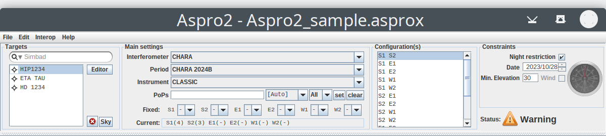
Period(VLTI / CHARA only) - Select the
Instrumentamong available instruments for the selected interferometer (and period) PoPs(Pipes Of Pan) configuration (CHARA only):- the text field let you define a specific PoPs combination (PoP 1 to 5) by giving the list of PoP numbers (1 to 5, 8 means any PoP) in the same order than stations of the selected configuration. If you leave this field blank, ASPRO 2 will determine "best PoP" combinations maximizing the observability of your complete list of targets. For example:
- VEGA_2T with baseline " S1 S2", "34" means PoP3 on S1 and PoP4 on S2
- MIRC (4T) with baseline "S1 S2 E1 W2", "1255" means PoP1 on S1, PoP2 on S2 and PoP5 on E1 and W2
- the combo box indicates if the current PoP combination is "Manual" (user defined) or "Auto" (best PoPs algorithm) and contains first best PoP combinations followed by up to 15 good PoP combinations (descending order). If you select one of its PoP combinations, the text field is updated and the observability is computed to let you see the impact of this specific PoP combination.
- Since ASPRO2 22.03, PoPs can be defined per station using the
Fixedcombo boxes (1 to 5 corresponds to PoP1 to 5, '-' means any PoP) that are used to restrict PoP values used by the "best PoP" algorithm. Using Fixed PoPs allows to compare multiple configurations (or baseline limits) in a consistent manner. Please use the button 'set' to copy the Current PoP combination and the button 'clear' to reset the Fixed PoP combo boxes. - The
CurrentPoP combination is displayed using the following format "Station(PoP number)..." and updated when the observability is computed.
- the text field let you define a specific PoPs combination (PoP 1 to 5) by giving the list of PoP numbers (1 to 5, 8 means any PoP) in the same order than stations of the selected configuration. If you leave this field blank, ASPRO 2 will determine "best PoP" combinations maximizing the observability of your complete list of targets. For example:
Configuration(s)
This panel let you choose one or more base line configurations in the configuration list which contains only available baselines for the selected instrument (and period for VLTI or CHARA).
To select several configurations, use the Control key or Command key (mac) before clicking on one configuration.
[!NOTE] As a convention, we will use the terms "single configuration" when only one configuration is selected and "multi configuration" when more configurations are selected.
See the Multi configuration support topic for more information.
Constraints
The Night restriction check box is useful to use or not night limits in the observability computation for a particular observation date. If disabled, it gives the largest observability intervals to see when the target is observable during the year.
An observation Date must be defined to determine the coming astronomical night and twilight zones used by the observability computation.
The date syntax uses the English format i.e. "YYYY/MM/DD".
For a given date, ASPRO2 determines the coming night range(s) in the [DD; DD+1] range; for example the given date '2014/4/4' corresponds to the night between April 4th and 5th.
The Minimum elevation must be given in degrees (45 degrees by default) to respect observation constraints on telescopes (at least 30 degrees).
Finally the Wind check box can be used during VLTI observations (on site) to define the wind direction used to determine the correct observability due to VLTI pointing restrictions.
[!NOTE]
- The default minimum elevation can be defined in the Preferences Window.
- ASPRO2 interprets the given date to determine the coming astronomical night in the [DD; DD+1] range.
Status indicator
The status (OK, Information or Warning) gives you the feedback on underlying computations: observability, UV coverage, OIFits data simulation and noise modelling.
Pointing the Information or Warning indicator with your mouse displays a tooltip containing status messages:
- Observability:
- info: (loaded obs. setup: ...)
- info: Baseline: ... - Beams: ... - PoPs: ... - Delaylines: ...
- info: The target [...] is not observable
- info: The target [...] is not observable (never rise)
- info: Target [...] is [not / partially] observable [HA or Moon or Wind restrictions]
- info: Equivalent Best PoPs found: (PoPs combinations) ...
- info: Next good PoPs: (up to 15 PoPs combinations) ...
- warning: Daylight Saving Time (DST) transition: observability ranges may appear shorter / longer !
- warning: Impossible to find a PoPs combination compatible with any observable target
- warning: Impossible to find a PoPs combination compatible with all observable targets (... / ...)
- warning: Moon separation is ... deg at HH:MM for target [...] Please check pointing restrictions
- warning: Pupil correction problem: VCM > [2.5|2.75|3.0] bar pressure limit exceeded.
- UV coverage:
- warning: Check your HA min/max settings. There is no observable HA
- warning: Too many HA points (...), check your sampling periodicity. Only 500 samples computed
- warning: Multiple configurations cannot be done in one night (night restrictions are only valid for YYYY/MM/DD)
- warning: User model [...] is disabled
- OIFits data simulation:
- info: ... instrument mode: ... channels [... - ... µm] (band: ... µm)
- info: User model [...]: ... images [... - ... µm] (increment: ... µm)
- warning: OIFits data not available
- warning: OIFits data computation is disabled
- warning: User model (Fits image) wavelength (... µm) outside of instrumental wavelength range
- warning: User model (Fits cube) without wavelength information is discarded
- warning: Incorrect model min wavelength [... µm] higher than max instrument wavelength [... µm]
- warning: Incorrect model max wavelength [... µm] lower than min instrument wavelength [... µm]
- warning: Incorrect model wavelength range [... - ... µm] smaller than the typical instrumental wavelength band [... - ... µm]
- warning: Sub sampling detected: ... channels but only ... user model images available
- warning: Restricted instrument mode: ... channels [... - ... µm]
- Noise modelling:
- info: Min O.B. time: ... s (... min) on acquisition - Ratio Interferometry: ... %
- info: Observation can take advantage of FT. Adjusting DIT to: ...
- info: Observation can take advantage of FT (Group track).
- info: Observation without FT. DIT set to: ...
- info: AO setup: ... in ... band
- info: FT associated to target [...]: ... mag
- info: AO associated to target [...]: ... mag
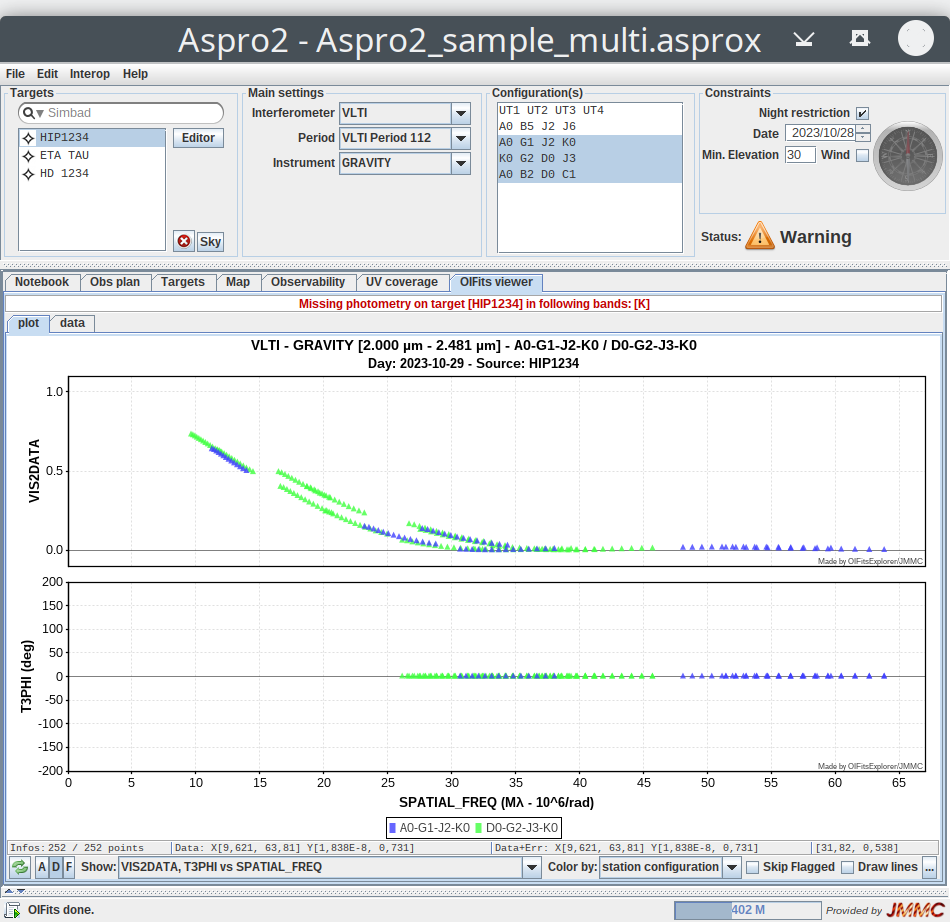
- warning: Missing photometry on target [...] in following bands: ... [instrument / fringe tracker / adaptive optics bands]
- warning: Missing photometry on FT target [...] in following bands: ... [fringe tracker band]
- warning: Missing photometry on AO target [...] in following bands: ... [adaptive optics band]
- warning: DIT too long (saturation). Adjusting it to (possibly impossible): ...
- warning: Observation can not use FT (magnitude limit or saturation)
- warning: Observation can not use AO (magnitude limit = ...) in ... band
- warning: Detector can not be read completely within 1 DIT: the wavelength range is restricted to ... µm
[!NOTE] clicking on the status opens the ASPRO 2 Log Console which displays the complete history of status messages
Targets tab
This tab brings all target's informations through a table view. Targets can be sorted by any column (use shift to add a second column ordering).
Click in the bottom right corner to choose your colums of interest.
Future release will improve the way to select, filter and group targets.
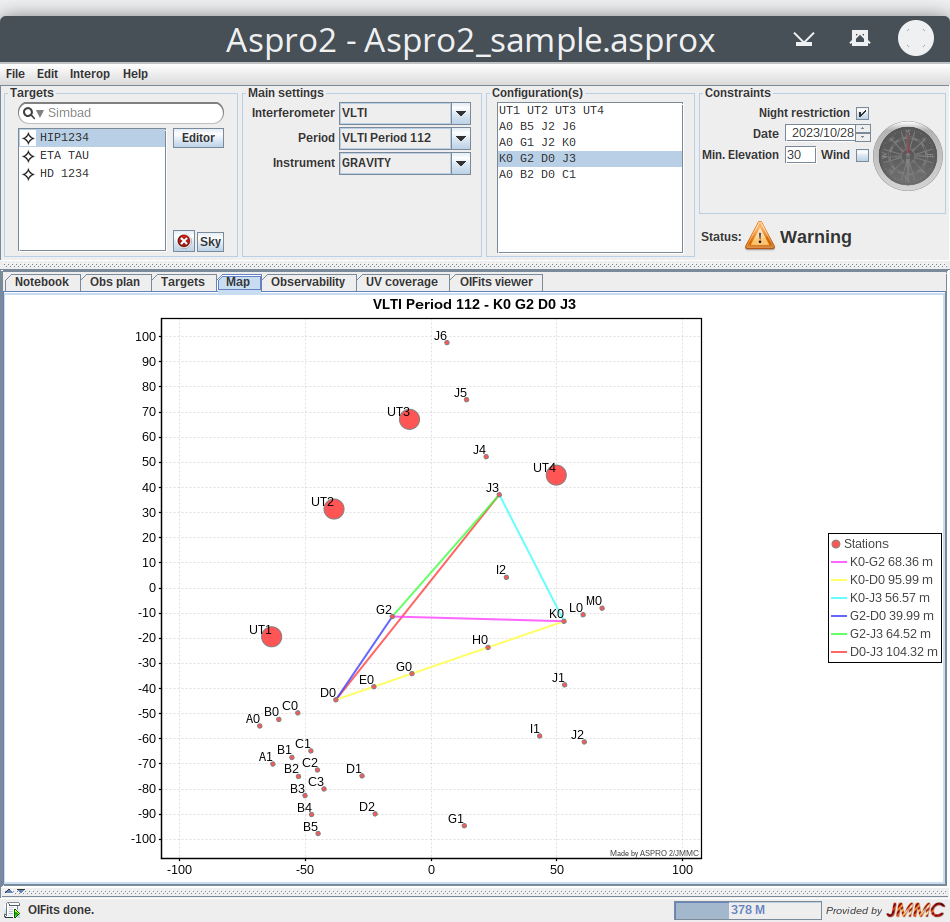
Interferometer sketch (Map tab)
This zoomable plot shows the selected interferometer with all stations and selected baselines. Selected baselines are indicated with their lengths in the legend area.
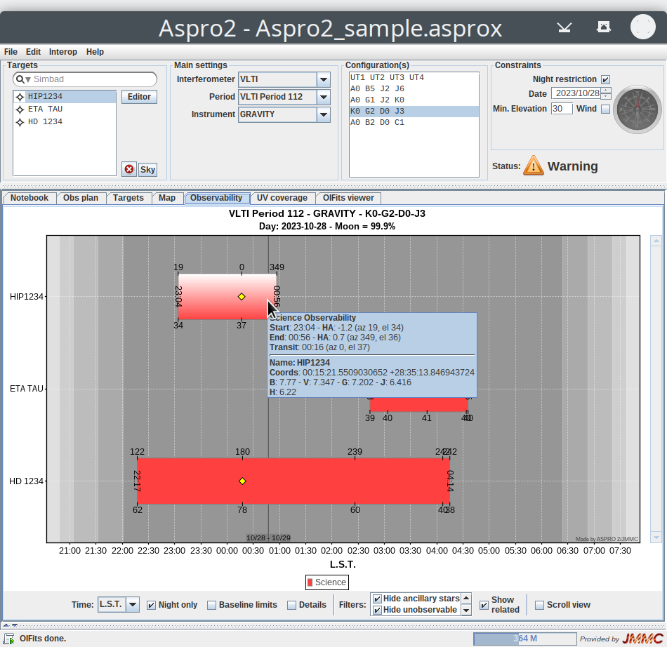
Observability tab
This zoomable plot shows the observability intervals per target expressed in LST, UTC or Local time for the chosen observation date.
A diamond mark indicates the transit of the target and graduation marks indicate the azimuth (on top: 0 means North, 90 means East...) and elevation (on bottom) of the target in degrees along the observability range.
If the night restriction is enabled, night and twilight zones for the chosen observation date are displayed in the background, used by the observability computation and the maximum FLI (Fractional Lunar Illumination) for this night is indicated in the chart title.
If your observation date corresponds to the current night, a red time line indicating the time is displayed and refreshed every minute.
Several plot options are available in this case:
- the plot is centered (by default) around night
- Use the
Night onlycheck box to display only the night (by default) - Use the
Scroll viewcheck box to adjust displayed targets:- If enabled, only few targets are displayed and the plot is scrollable (mousewheel supported) but the exported PDF always contains all targets (multiple page if necessary)
- If disabled, all targets are displayed and the plot can be zoomed in / out (mouse) but the exported PDF document contains targets as displayed (single page only)
- Use the
Filtersto show / hide targets:- Show groups: show only targets belonging to the selected
Groups(user-defined groups). - Hide calibrators: hide all targets flagged as calibrator and orphaned calibrators
- Hide ancillary stars: hide all targets (FT, AO, Guide stars) (see Groups )
- Hide unobservable: hide all targets that are not observable or never rise
- Use the
Show relatedcheck box (enabled by default) to show / hide the science and calibrator targets related to the selected target even if those targets are filtered
- Show groups: show only targets belonging to the selected
[!NOTE] The default time reference (LST, UTC or Local),
Center plot around night,Night onlyoptions and theTwilight used as night limit(astronomical, nautical or civil) can be defined in the Preferences Window.
Target observability takes into account:
- night limit for the observation date (if enabled)
- chosen minimum elevation
- delay line compensation for selected baselines
- CHARA'S Pipes Of Pan (PoPs), detailed below
- telescope shadowing (VLTI)
- zenithal restriction
- optional constraints (hints):
- HA constraints, defined in the UV coverage panel
- moon avoidance, detailed below
- wind direction (VLTI), detailed below (if enabled)
- VLTI constraints related to the Variable Curvature Mirror (VCM) pressure limit to 2.5 bar (before ESO Period 96): this constraint indicates that the pupil may be not well corrected (flux / FoV loss) and is represented by several pressure thresholds (2.5, 2.75 and 3.0 bar) as darkened areas on the target observability and indicated in its tooltip.
[!NOTE] the impact of optional constraints (HA, moon avoidance and wind restriction) on the target observability is displayed using a translucent area and dotted outline.
Colors are automatically associated to targets and their meaning is described in the legend area: (Science / Calibrator or configuration).
The selected target in the main target list is represented highlighted using a gradient (white to 'color') and the observability plot is automatically updated when the selected target changes.
[!NOTE]
- Clicking on a target on the observability plot updates the selected target in the target list and refreshes Observability, UV coverage and OIFits viewer plots.
- Pointing an observability interval with your mouse displays a tooltip containing interval information (start, end and transit time with their corresponding hour angle, azimuth and elevation), target information (name, coordinates and known magnitudes) and target notes if present (indicated by [i] in the target name).
- In case you have many targets, use the vertical scrollbar (or mouse wheel) to navigate among your targets when the
Scroll viewcheck box is checked; otherwise, all targets are displayed and use your mouse to zoom in / out..- You can use the
Editmenu /Findaction (Previous / Next) to find and select a target in the target list and find it on the observability plot.- You can sort your targets by their right ascension or manually in the Target Editor.
- Please set correctly your date / time settings on your machine (operating system) to let the time marker work properly.
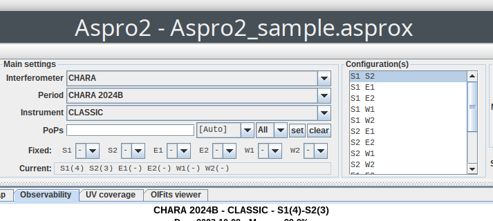
Show more details on the PoPs configuration and best PoPs algorithms:
ASPRO 2 finds the best PoPs combination for the complete target list when the PoPs text field is empty.
The current PoPs combination is indicated in the Current label, in the plot title and in status indicator messages using the following format "Station(PoP number)...", as in the following image:
You can use the PoPs combo box to list best PoP combinations followed by up to good PoP combinations (descending order) and select one to see its impact on the observability of your complete target list.
You can tell ASPRO 2 to use another PoPs combination by entering a valid PoPs code in the PoPs text widget ( "34" means PoP3 on S1 and PoP4 on S2), as in the following image:

To compare observability between 6T and 5T configurations, please use the Fixed PoPs combo boxes (and the set / clear actions) to associate PoPs with stations in a stable manner:
- once the best PoPs at 6T is found, use the
setaction to use it as Fixed values, as in the following image: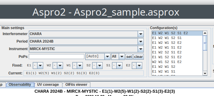
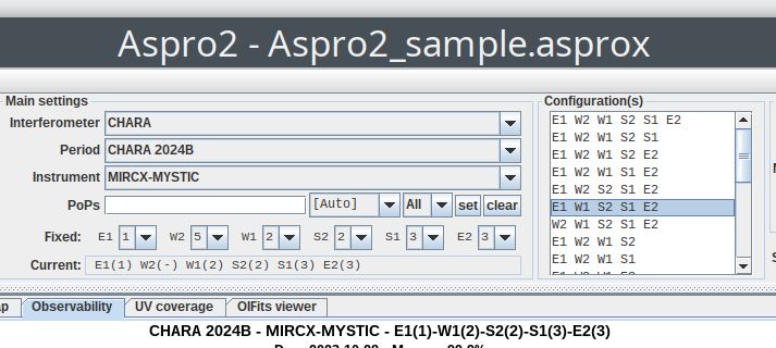
- you can then change the configuration (or select multiple ones) like a 5T configuration, as in the following image:
The best PoPs algorithm has two different behaviour depending on your target list:
- single target: the best PoPs corresponds to the PoP combination maximizing the total observability interval (sum of each observability interval).
- multiple targets: the best PoPs corresponds to a different solution: it uses an estimator that tries to maximize both total observability interval and longest minimal observability interval among all targets in order to be able to observe all targets = a PoP combination giving better observability for a subset of targets can be discarded if it leads to unobservable target(s).
The best PoPs algorithm takes only into account (for performance reasons):
- night limit for the observation date (if enabled)
- chosen minimum elevation (rise/set interval)
- delay line compensation for selected baselines
- HA constraints (not in the Simple algorithm)
- Fixed PoPs restrict the evaluated PoP combinations (W2 is set to Pop5 by default)
Finally, the best PoPs algorithm has several variants:
- Simple (former algorithm used until ASPRO 2 0.9.4 release)
- Transit: maximizes the observability interval arround transit
- HALimits: maximizes the observability interval within HA constraints(lower and upper hour angle)
Both Transit and HALimits variants use a normal law estimator (mean, standard deviation). cas de sélection, une phase A en 2028. L’ESO insiste sur la notion de roadmap qui intégrerait plusieurs propositions distribuées dans le temps.’ Several options can be defined in the Preferences Window:
Best Pops algorithmamong variants: Simple, Transit, HALimitsGaussian sigma(Transit and HALimits only) to adjust the selectivity of the normal law (transit or HA range confidence)Average weight % Minto adjust the importance of the shortest observability interval (min) compared to the average observability interval for your complete target list
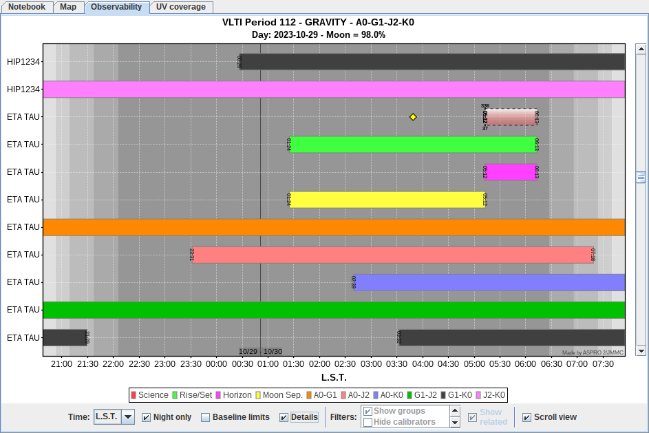
Show more details on the observability computation:
The detailed observability plot shows each target multiple times (look at the legend area) to illustrate different aspects:
- Rise/Set intervals indicate when the target is above the chosen minimum elevation and respects the night restriction (if enabled)
- Horizon intervals indicate when the target is not affected by shadowing restrictions (VLTI) and zenithal restriction
- Moon Separation intervals indicate when the target is not affected by moon avoidance
- Wind intervals indicate when the target is not affected by pointing restrictions due to the wind direction (azimuth)
- Individual Base line intervals indicate when delay lines can compensate the optical path difference between two stations
Show base line limits for the selected configuration:
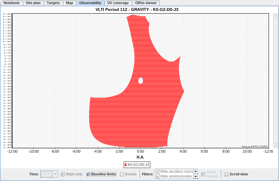
This plot is useful to see telescope shadowing restrictions for the selected baselines on the VLTI and also the zenithal restriction.
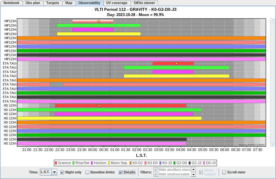
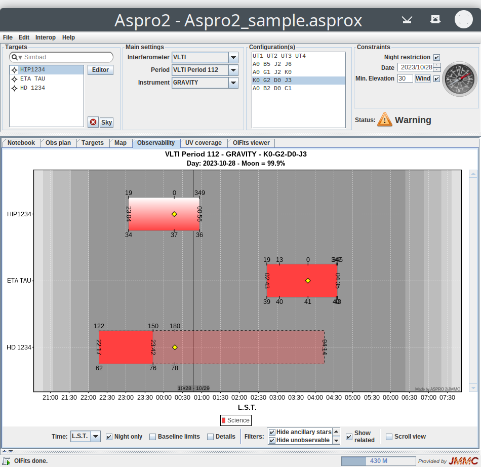
Show more details on the moon avoidance:
ASPRO 2 determine the moon separation with every target during the rise / set interval only.
Here are the rules for each interferometer:
- CHARA and SUSI: moon separation > 5 degrees
- VLTI: moon separation > 1 degrees
- UTs: if the FLI is > 85%,
- moon separation > 10 degrees if the V flux < 9.0 mag
- moon separation > 20 degrees if the V flux > 9.0 mag
- ATs: if the FLI is > 95%,
- moon separation > 3 degrees if the R flux < 9.0 mag
- moon separation > 5 degrees if the R flux > 9.0 mag
- UTs: if the FLI is > 85%,
On the following screen shot, the target ETA TAU is not observable because it is too close to the moon (~ 2.1 deg) at this particular date (2015/10/28).
Show more details on entering the VLTI wind direction:
When the Wind check box is enabled (night restriction should be enabled first), the compass widget is also enabled to let you enter the wind direction represented by the red arrow.
On this screen shot, the wind direction is set to North - East (60 deg) and the target HD 1234 is impacted (telescopes can not be pointed to South - West).
Here is the detailed observability plot in this case when the Details check box is then enabled:
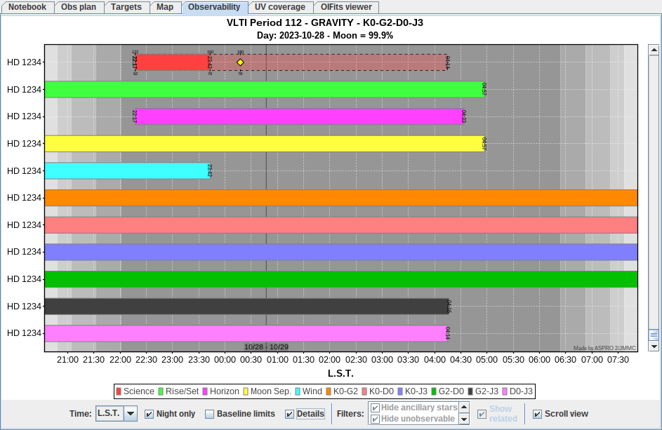
The observability interval related to Wind pointing restriction is represented in cyan color and is the limiting effect on the target HD 1234.
UV coverage tab
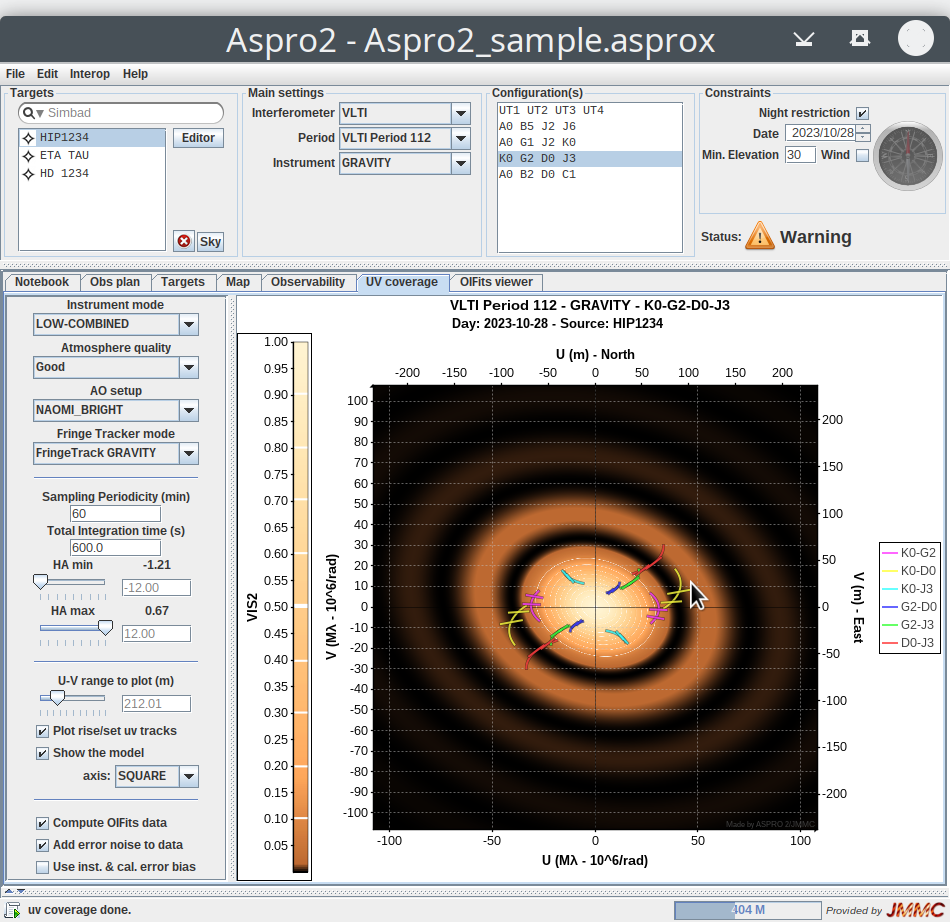
This zoomable plot shows the UV coverage for the target selected in the target list of the main panel.
An optional image of the target object model is displayed on the background which represents the amplitude, square amplitude, phase of the Fourier transform of the target model and its color scale (linear or logarithmic) is displayed on the left side. You can use the Add error noise to image in the Preferences Window to perform noise modelling (VIS or VIS2) and add error noise to the model image.
It can show UV tracks per base line given by the Rise / Set intervals only to see the largest elliptical paths supporting UV measurements.
UV measurements are represented by UV segments as the spectral resolution is simulated for the selected Instrument mode (wavelength range).
If your observation date corresponds to the current night, red segments indicating current UV measurements and the LST (or UTC) time are displayed and refreshed every minute.
These UV measurements are using the observability range of the target expressed in hour angle displayed near the HA min and HA max sliders and the Sampling Periodicity in minutes (default value depending on the chosen instrument). Besides, these hour angle fields are useful to adjust the starting and ending hour angles of the simulated observation.
Important actions:
- Export to OIFits: Observables (VIS, VIS2, T3) are simulated with error and noise modelling (if enabled) and can be exported to an
OIFits file using the
Filemenu /Export to OIFits file(s)action or in multi configuration mode to 1 merged OIFits file (all configurations). - Export to Observing blocks : export as XML files using the
Filemenu /Export to an Observing Block (XML)orInteropmenu /Send Obs. Block(s) to A2P2actions.- a2p2 handles such files for VLTI observations, Observing blocks compatible with ESO P2 tools can be generated for the selected target and its calibrators
- a2p2 handles CHARA observations providing a log record for the selected science target and ancillary data.
On the following screen shot, the object model is an elliptical uniform disk which visibility amplitude is converted using a linear scale: 0.0 is indicated in black and the maximum (1.0 because fluxes are normalized) in white.
[!NOTE]
- Pointing an UV segment with your mouse displays a tooltip containing the information (configuration, baseline, current time / hour angle, UV radius and position angle).
- The model image resolution (256 x 256 up to 2048 x 2048), its color table (LUT) and color scale (linear or logarithmic) can be chosen in the Preferences Window.
On the left side, many options are proposed:
Instrument mode: the proposed choices depend on the selected instrument, corresponding to the different offered combinations [beam combiner, spectrograph (Prism or Grism), spectral resolution (High, Medium or Low), wavelength range]AO setup: this gives the offered configurations of the Adaptive Optics (MACAO or CIAO on UTs, NAOMI on ATs), used by the noise modelling to compute the Strehl ratio in the AO bandAtmosphere quality: used by the noise modelling, it represents the following sky conditions (followed by the percentage of night time according to ESO at Paranal Observatory):- EXCELLENT: Seeing < 0.6 arcsec, t0 > 5.2 ms (10%)
- GOOD: Seeing < 0.7 arcsec, t0 > 4.4 ms (20%)
AVERAGE: Seeing < 1.0 arcsec, t0 > 3.2 ms (50%)- WORSE: Seeing < 1.15 arcsec, t0 > 2.2 ms (70%)
- BAD: Seeing < 1.4 arcsec, t0 > 1.6 ms
- AWFUL: Seeing < 1.8 arcsec, t0 > 0.5 ms
Fringe tracker mode: used by the noise modelling to adjust the detector integration time if the Fringe Tracker is present.Sampling Periodicity: indicate the time in minutes between two (SCI) measurementsTotal integration time: indicate the effective time in seconds to repeat and integrate measurements on the (SCI) detectorWL Ref.: (optional) indicate the central wavelength to define the wavelength range read on the (SCI) detector (cas de sélection, une phase A en 2028. L’ESO insiste sur la notion de roadmap qui intégrerait plusieurs propositions distribuées dans le temps.’MATISSE Medium / High resolution without GRA4MAT) when the full detector cannot be read within 1 DITHA minandHA maxfields: use either sliders or numeric text fields to enter the starting and ending hour angles in order to restrict the hour angle range where UV measurements are taken (used by Observability computation, OIFits simulation and Observing blocks)U-V range to plot: define the U-V range in meters to use in the plot rendering and model image computation (related to the plot scale)Plot rise/set uv tracks: If enabled, UV tracks are displayed to show the elliptical paths supporting UV measurements given by the Rise / Set intervals of the selected targetShow the model: If enabled, an image representing the Fourier transform of the target's model is displayed on the background of the UV planaxis: you can choose to represent the amplitude (AMP), phase (PHASE) or square amplitude (SQUARE) of the Fourier transform of the target's model- For polychromatic user-models (Fits cube only), a slider is displayed to navigate among model images (or cycle automatically
through them using the
Autobutton) and refresh the displayed Fourier transform of the target's model Compute OIFits data: enable / disable the computation (in background) of the simulated OIFits dataAdd error noise to data: enable / disable error noise on observables of the OIFits data; errors are still computed. The default value can be set in the Preferences WindowUse inst. & cal. error bias: if enabled, the noise modelling adds the instrumental visibility / phase & calibration biases to OIFits data error; if disabled, only the theoretical instrumental noise is taken into account
[!NOTE]
- As this plot is zoomable, do not hesitate to zoom in and see if the UV coverage on your object model is interesting.
- When an user-defined model is used (FITS image), the Fourier transform is computed using an optimized Fast Fourier Transform algorithm of the given image using the best FFT kernel size (zero padding) to obtain a model image size close to the chosen model image resolution in the Preferences Window; however, if it is too slow, consider using the
Fast mode (optimize the input image)in the Preferences Window or reducing either the model image resolution or the input image resolution or size.- In this case, the zoom feature only performs model image zoom (pixels) and do not recompute the Fourier transform to get more details; use the
U-V range to plotto force ASPRO 2 to compute the Fourier transform again or use an higher model image resolution.- When an user-defined model is used (FITS image), OIFits data are computed using direct Fourier transform (not FFT) which can be slow (high resolution) but more precise at each UV point; however, if it is too slow, consider using the
Fast mode (optimize the input image)in the Preferences Window or disable OIFits data computation when not absolutely needed.
OIFits Viewer tab
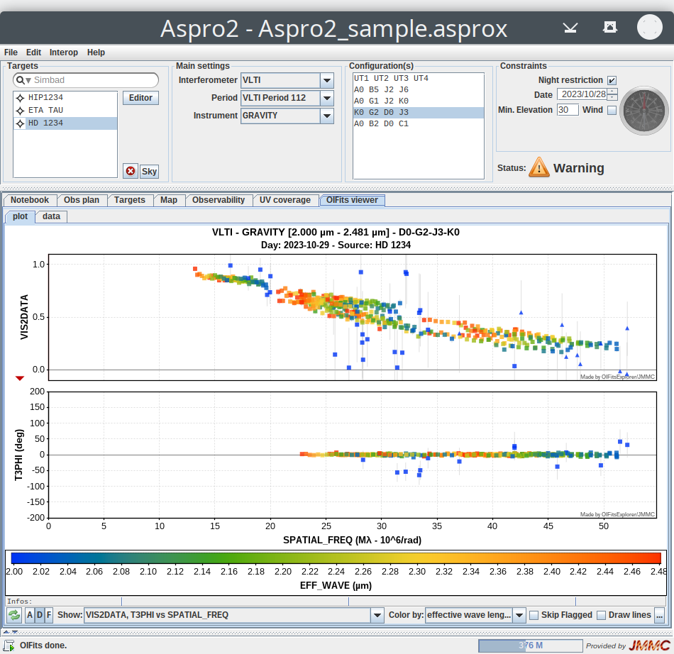
The OIFits viewer uses an embedded OIFitsExplorer which provides several predefined but customizable plots showing the OIFits simulated data (VIS, VIS2, T3, FLUX) only if the target has an object model and the OIFits data computation is enabled on the UV coverage panel.
The Show combo box lists many predefined plots:
- VIS2DATA_T3PHI/SPATIAL_FREQ: square visibility (VIS2DATA) and closure phases (T3PHI) vs the spatial frequency (or its maximum for closure phases)
- VIS2DATA_T3PHI/EFF_WAVE: square visibility (VIS2DATA) and closure phases (T3PHI) vs the wavelength of the spectral channel
- VIS2DATA_T3PHI/MJD: square visibility (VIS2DATA) and closure phases (T3PHI) vs the modified julian day
- VISAMP_VISPHI/SPATIAL_FREQ: visibility amplitude (VISAMP) and phase (VISPHI) vs the spatial frequency
- LOG_VISAMP_VIS2DATA/SPATIAL_FREQ: visibility amplitude (VISAMP) and square visibility (VIS2DATA) using logarithmic scale vs the spatial frequency
- etc ...
The Color by selector allows to color data points by effective wavelength, baseline or configuration (multi-configuration).
The Skip flag data checkbox is important to filter out simulated data having signal to noise ratio SNR < 3 (high uncertainty), that may occur at instrument wavelength boundaries. Ths threshold value (3 by default) can be set in the Preferences Window.
The Draw line checkbox allows to plot lines along the wavelength axis instead of data points to observe the spectral dispersion; if the x axis corresponds to EFF_WAVE (wavelength), then step lines are used to display histograms (spectra like).
To customize the plot axes, please use the [...] button to select the plotted axes / quantities (among OIFITS data columns) and define their ranges (auto / fixed) and many other options (log, include zero).
The plot includes error bars representing the error computed by the noise modelling.
There are 2 types of "noise" in Aspro2:
- the first one is the noise associated to a single observation and is directly caused by the numbers of photons available for "fringe detection" on the instrument detector. It will decrease with the brightness of the source and the transmission of the telescopes, delay lines, instrument, exposure time (more photons available to start with). It will increase with the detector noise and the atmospheric turbulence.
- the second (and often dominant) one is just an added percentage of error expected on calibrated values, accounting for the variation of seeing, flux etc between the science target and its calibrator. This latter "noise" can be deactivated in the interface.
Data and errors are coming from the simulated OIFits file generated "on the fly" which can be exported using the File menu / Export to OIFits file action.
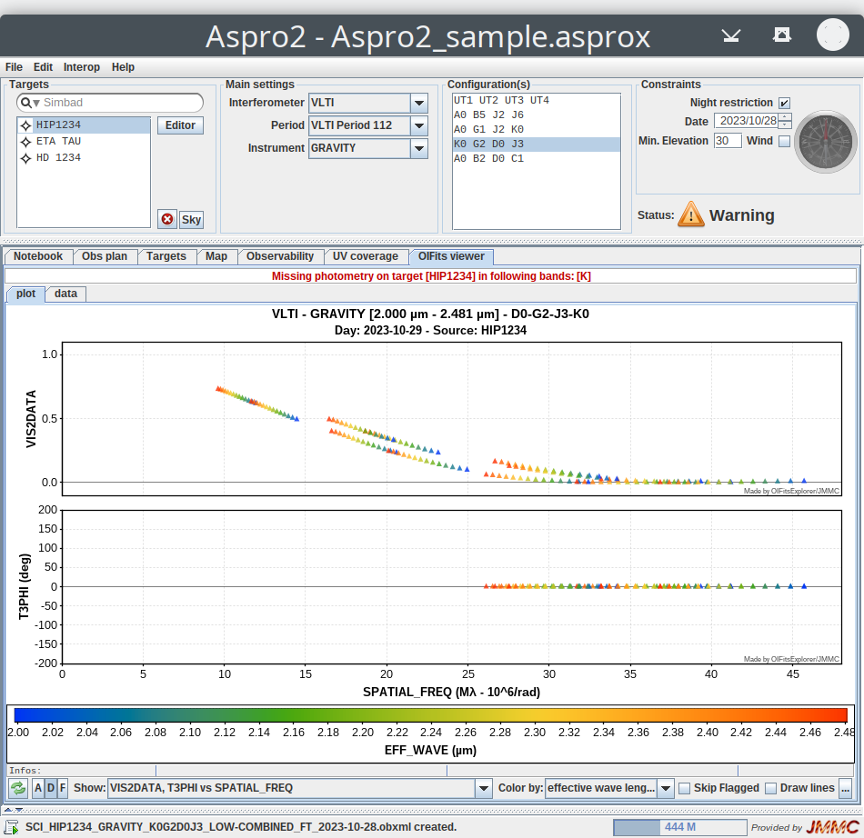
[!NOTE] If errors can not be computed by the noise modelling (missing target magnitudes...), data points are then represented using a triangle shape and of course, error bars are not displayed:
[!NOTE] To enable / disable the OIFits computation or error noise, look at the UV coverage panel. When an user-defined model is used (FITS image), OIFits data are computed using direct Fourier transform (not FFT) which can be slow (high resolution) but more precise at each UV point; however, if it is too slow, consider using the
Fast mode (optimize the input image)in the Preferences Window or disable OIFits data computation when not absolutely needed in the UV coverage panel.
OIFits output
ASPRO 2 generates OIFITS (version 1) compliant files for the select target using the current observation setup with OI_VIS, OI_VIS2, OI_T3 and OI_FLUX tables. The OI_FLUX table (OIFITS version 2) gives the theoretical target's flux in photons (no atmosphere nor transmission loss, strehl).
To illustrate the bandwidth smearing effect of the instrumental spectral configuration, ASPRO 2 uses super sampling (3 samples by default) on the target model to compute complex visibilities for instrument modes having less than 100 spectral channels (large bandwith).
The noise modelling can estimate errors on OI_VIS, OI_VIS2, OI_T3 and OI_FLUX data based on object magnitudes and the current instrument configuration and observation setup (fringe tracker, adaptive optics...).
If a magnitude or flux is missing, errors can not be computed:
- the OIFits error column is filled with
NaNvalues and marked as invalid (flags = T) - the status is Warning in ASPRO 2 with an appropriate message.
[!NOTE]
- The number of samples used by the super sampling can be defined by the
Supersampling model in spectral channelsin the Preferences Window.- The OI_VIS table contains additional (non-standard) columns VISDATA and VISERR to store correlated fluxes as complex data;
About VISAMP and VISPHI quantities in OI_VIS tables:
- These quantities gives the amplitude and phase of either absolute or differential complex visibilities depending on the selected instrument as described by the OIFITS 2 standard.
- The differential visibility is the object complex visibility divided by a reference complex visibility : C_diff_vis(lambda) = C_vis(lambda) / C_vis_ref(lambda).
- This reference visibility in Aspro2 is the mean of all spectral channels (except the one considered): C_vis_ref(lambda) = ( Sum[ C_vis(l) ] - C_vis(lambda) ) / (N - 1).
- Differential VISAMP are then normalized by mean(VISAMP) of all spectral channels so it can exceed 1 i.e. only visibility variations with respect to the reference visibility is meaningful, typically to analyse an absorption line.
- The keywords AMPTYP/PHI_TYPE contains the 'absolute' or 'differential' value to indicate how the VISAMP and VISPHI quantities were computed.
- The Status Indicator also displays this information 'OI_VIS: (Differential/Absolute) VisAmp - (Differential/Absolute) VisPhi")'.
- The following table lists instruments using differential complex visibilities in ASPRO2:
| Instrument | VISAMP type | VISPHI type |
|---|---|---|
| AMBER | differential | differential |
| GRAVITY | differential | differential |
| MATISSE | absolute | differential |
Noise modelling is based on the JMMC-MEM-2800-0001 - Noise model for interferometric combiners document.
In 2016, the noise modelling and the OIFITS data simulator has been improved for new VLTI instruments (GRAVITY & MATISSE) and this work has been described in the SPIE proceedings: L. Bourgès and G. Duvert, “ASPRO2: get ready for VLTI’s instruments GRAVITY and MATISSE”, Proc. SPIE 9907, Optical and Infrared Interferometry and Imaging V, 990711
Since ASPRO2 2024.03 noise modeling has been improved:
- enhanced AO model for GRAVITY+ GPAO Natural Guide Star (NGS) to estimate the Strehl ratio and the isoplanetism error using distances between the AO target and interferometric targets (GRAVITY FT or SCI). This implementation was made in collaboration with Dr. Anthony Berdeu, LESIA, ObsPM, whose project has received funding from the European Union's Horizon 2020 research and innovation programme under grant agreement No 101004719.
- implemented the visibility loss for off-axis fringe tracking (GRAVITY FT): it includes the Coherence loss due to phase jittering during fringe tracking and the off-axis coherence loss due to the atmospheric anisoplanetism. To determine the overall visibility loss, an observation with the instrument GRAVITY_FT (automatic DIT based on SNR) is first simulated (LOW mode, 6 channels) to compute the Signal-To-Noise ratio on the FT target (if defined) using its own model (or V=1 if undefined). The SNR per baseline estimation is the weighted average over spectral channels and the bootstrapping for baselines (triangle method) is applied. The RMS variation of the residual optical path differences (OPDs) is derived from the SNR per baseline and FT parameters (automatic DIT & vibration RMS) to give the RMS variation of the fringe phase on the GRAVITY (SCI) detector per baseline and spectral channel. The DIT is automatically determined to use the longest possible DIT that avoids the detector saturation. This implementation was made in collaboration with Dr. Taro Shimizu, MPE (GRAVITY+ Simulator, private communication on his note and python code).
See ASPRO2 - How to prepare VLTI's GRAVITY or MATISSE observations with new GPAO ?
Noise modeling plots:
- AO Strehl ratio per instrument:
- GRAVITY_FT SNR vs magnitude on ATs / UTs
The relevant parameters for each instrument are described in: Latest Aspro Configuration
Get Information about past observations
Since ASPRO2 release 20.03, ASPRO2 can retrieve past observations logs from the JMMC ObsPortal service. It provides observations logs from the ESO archive (all VLTI instruments) with lots of details: observation setup (configuration, instrument mode), date & time, UV points & atmospheric conditions.
To get observation logs for a single target, first select the target and use the Edit menu / Get Observations (Selected) action. To get observations logs for all targets, use the Edit menu / Get Observations (All targets) action. Depending on the number of targets and the amount of downloaded data, this action can take a while.
If any past observation corresponds to the selected target, a data table will be displayed on the bottom of the main window showing the corresponding data.
To filter these data, the table panel provides (several) filters:
- instruments: 1 or multiple instruments can be selected to only display the corresponding observation logs.
- (more filters will be added in the future)
[!NOTE]
- The query performs a cone-search with a radius of 30 as, so it may retrieve observations from different objects.
- Please use the
cancelbutton in the status bar to cancel any pending HTTP request.
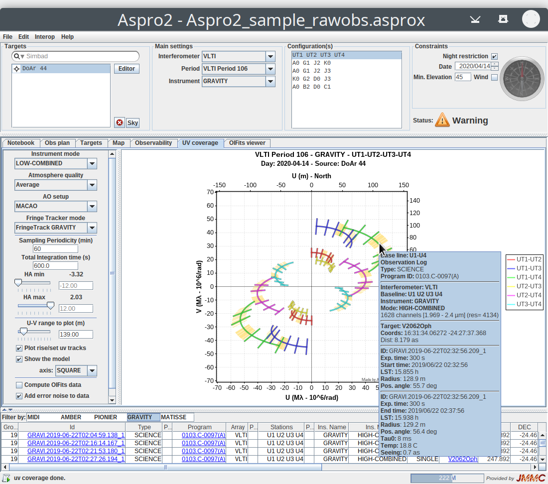
Observability plot
This plot shows the observability plot of the target 'DoAr 44'.
Past observation ranges of the GRAVITY instrument are displayed as an overlay in orange color:
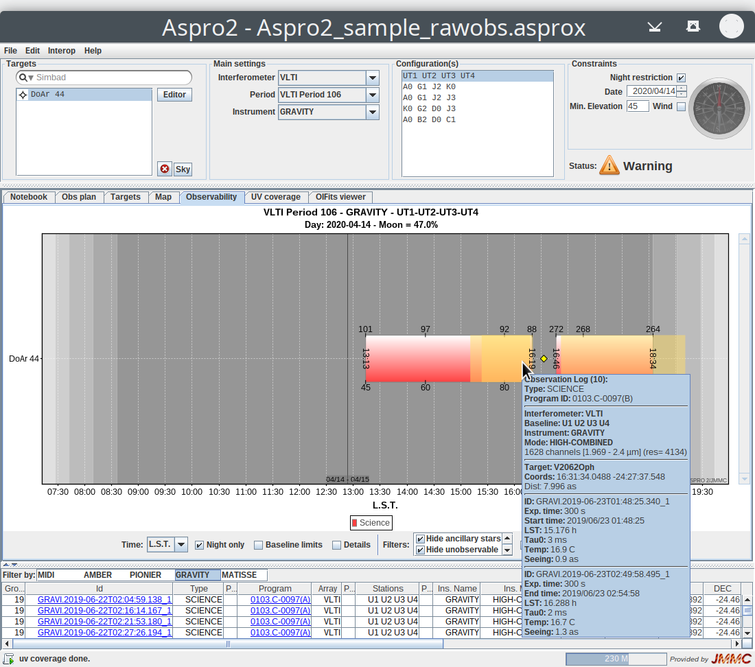
'V2062 Oph' and 'DoAr 44' are the same object in Simbad, even if the distance between the ASPRO2 target coordinates and the observation coordinates in the ESO archive is 8 as in this specific case.
[!NOTE] Tooltips are showing details about the pointed observation log.
UV Coverage plot
This plot shows the UV coverage of the target 'DoAr 44'. Past observation UV points of the GRAVITY instrument are displayed (in the background) in orange color:
[!NOTE] Tooltips are showing details about the pointed observation log.
Multi configuration support
When several configurations are selected in the Configuration(s) list, ASPRO 2 evaluates all configurations and updates plots accordingly.
This behaviour corresponds in the real world to perform multiple observations of one target using the same observation settings but using different configurations; these observations are done during several nights: switching from one configuration to another is not allowed during the night.
If night restrictions are used in multi configuration mode, the following warning appears: "Multiple configurations cannot be done in one night (night restrictions are only valid for YYYY/MM/DD)". Night and twilight zones are still helpful to know roughly when these observations can be planned.
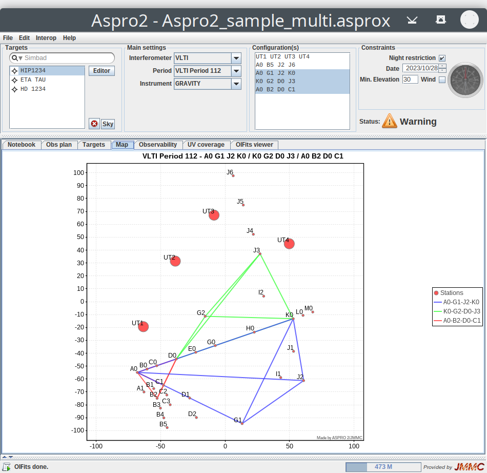
To illustrate this feature, following configurations are selected to produce the plots below:
- UT1 UT2 UT3
- B2 D0 C1
- K0 G2 D0
[!NOTE]
- Plots share the same colors associated to selected configurations which are indicated in the legend. For CHARA observations, the legend indicates the "best PoP" combinations found for each configuration.
Interferometer sketch
This plot shows selected configurations and their related baselines:
Observability plot
This plot represents the observability intervals per target and configuration:
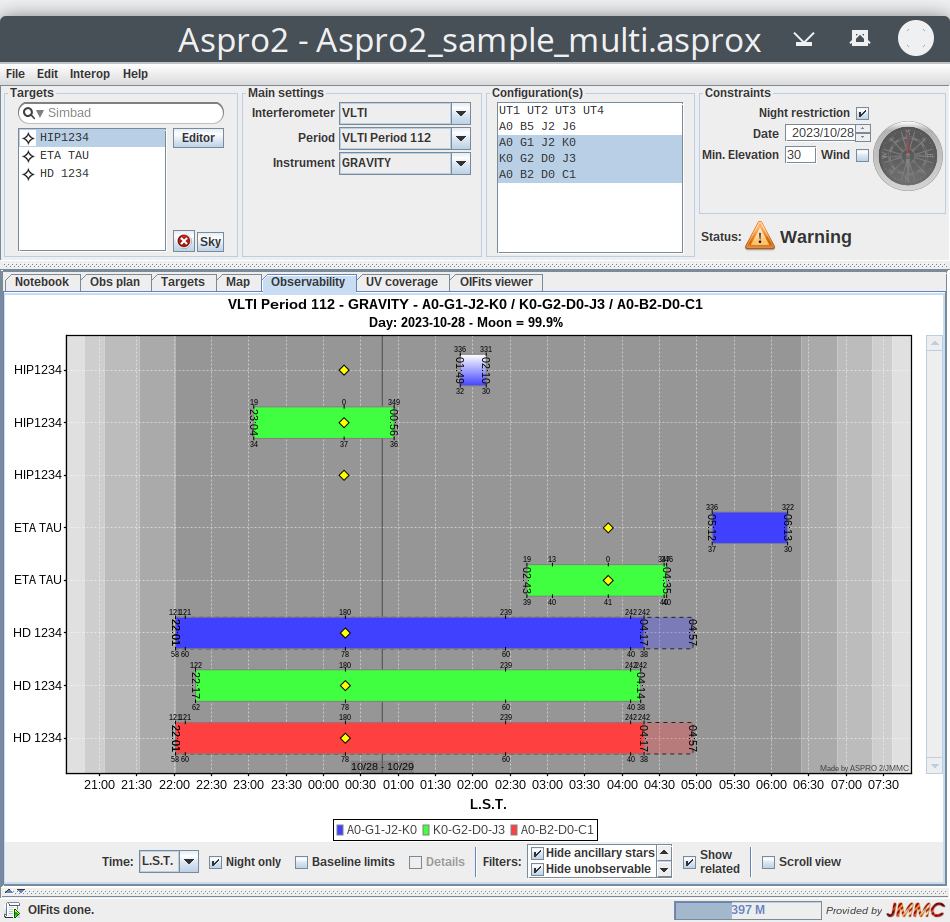
[!NOTE]
- Science and calibrator targets are represented using the same color; but names of calibrator targets have the "(cal)" suffix.
- Only the
Detailscheck box is disabled in Multi configuration mode- Use the vertical scrollbar (or mouse wheel) to navigate among your targets.
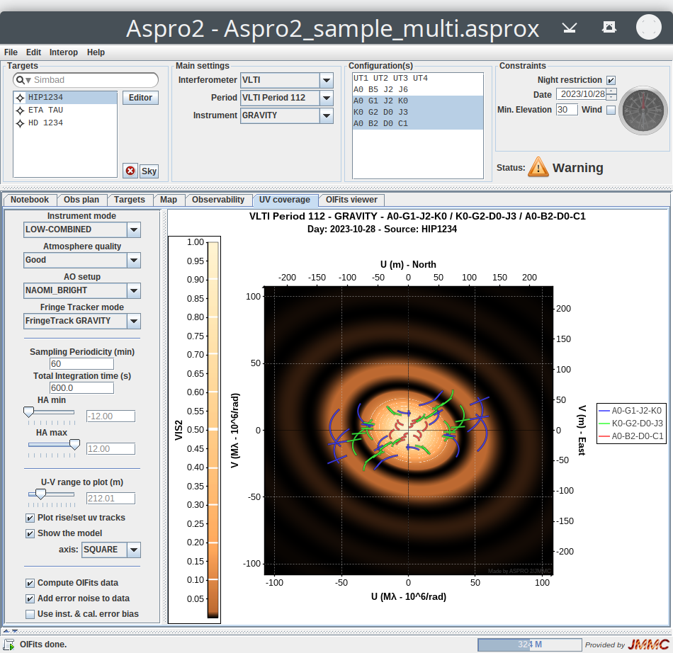
UV Coverage plot
This plot shows the combined UV coverage of your target using selected configurations:
OIFits viewer
This plot shows the combined OIFits data of your target using selected configurations:
Target Editor
This window provides 3 tabbed panes respectively to edit target information, target object models and target groups & associations.
[!NOTE]
- To help you navigating among targets, when you select a target in one tabbed pane, it is also selected in other tabbed panes.
- This window is modal i.e. changes are only effective when you click on the
OKbutton; closing the window or clicking on theCancelbutton is equivalent
Targets Tabbed Pane
The Targets panel allows you to edit target information and associate calibrator target(s) to your science target(s).
On the first screen shot, only science targets are present; on the second screen shot, science and calibrator targets are present:
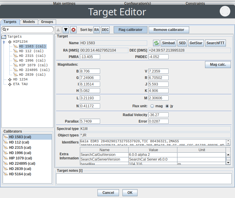
In the tree view on the left, targets are shown using the following rule to order targets: science targets followed by their calibrator targets.
In the calibrator list on the bottom left, all calibrator targets are present only once. On the right, the target information of the selected target is displayed and can be edited.
[!NOTE]
- Both the target tree and the calibrator list support "Drag and Drop" to let you associate one calibrator target to one science target:
- You can drag a calibrator from the calibrator list and drop it to any science target present in the target tree.
- Besides inside the target tree, you can use the
Controlkey orCommandkey (mac) to copy a calibrator target from one science target to another one; by default, the calibrator target is moved.
To sort both your science and calibrator targets by their right ascension (R.A.), click on the Sort by R.A. button.
To sort manually your science or calibrator targets, use up or down buttons to move:
- one science target (and its calibrators) among science targets
- one calibrator target among the calibrator targets of the same science target
To add a new target, use the Simbad star resolver to resolve target(s) by their identifier (see Targets).
To remove the current target, use the small "X" button and confirm the operation. If the selected target is a:
- science target, its associated calibrators are not removed automatically
- calibrator target, it is also removed automatically from every calibrator list of your science targets
To flag a science target as a calibrator target, select first a science target in the tree view and then click on the Flag calibrator button to enable it: this target is then moved from the tree view to the calibrator list and can be later associated to other science targets using "Drag and Drop". Of course, it is not possible to flag a science target that already has any calibrator target.
Objects can have other flags to be used as Adaptive Optics, Fringe Tracker or Guide stars, see Groups.
To remove the calibrator flag from a calibrator target, select first a calibrator target either in the tree view or in the calibrator list and then click on the Flag calibrator button to disable it: this target is then moved from the calibrator list to the tree view. Of course, if this calibrator target is already associated to science targets, a confirmation message is displayed "Do you really want to remove associations with this calibrator ?". If you confirm, it is also removed automatically from every calibrator list of your science targets.
To remove a calibrator target from the calibrator list of one science target, select first this calibrator target in the tree view and then click on the Remove Calibrator button.
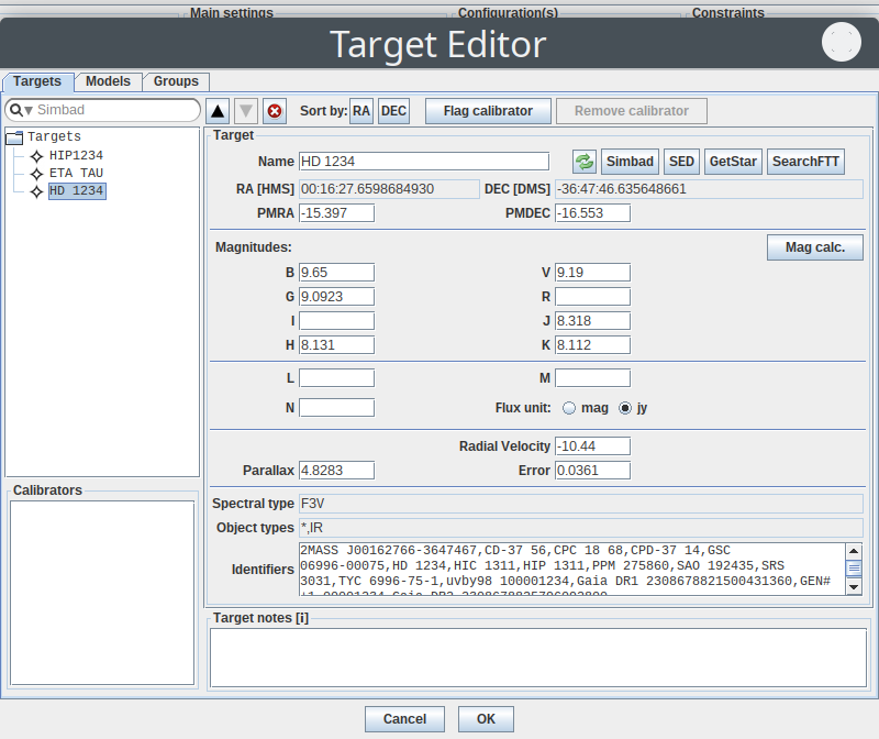
The Target form let you see target information and edit some fields:
- Target Name, RA / DEC coordinates (in HMS / DMS format); click on the
Simbadbutton to open the CDS Simbad web page, on theSEDbutton to open the CDS SED explorer, on theGetStarbutton to open the JMMC GetStar page corresponding to this target - PMRA / PMDEC: proper motion in mas/yr (only used by Observing blocks and OIFits format)
- Magnitudes: contains known object magnitudes in B-V-G-R (visible), I-J-H-K L-M-N (infrared) bands; you should fill these values when the noise modelling reports missing target magnitude(s). L-M-N fluxes can be expressed in Jansky (Jy) or mag.
- Radial velocity in km/s, Parallax in mas and its Error in mas/yr (only used by Observing blocks and OIFits format)
- Spectral type, Object types and Identifiers from CDS Simbad catalogs (read only)
- Extra Informations available only for SearchCal calibrators or VOTable interoperability: this table presents main parameters and fields computed by SearchCal including diameters (uniform disk diameters per band...) or provided by external tools
The Target notes field let you edit user comments about the selected target.
Models Tabbed Pane
The Models panel allows you to edit the object model of your targets using either an analytical model or an user-defined model (FITS image).
For the selected target, choose the correct Mode to enable its Analytical or User model.
In the tree view at the top left, targets with their models are shown using the following rules to order targets:
- science targets first
- then calibrator targets
[!NOTE]
- Calibrator targets are present only once in the tree view and are not associated to their science target in this view.
- SearchCal calibrators have an uniform disk model whose diameter can be edited in this panel.
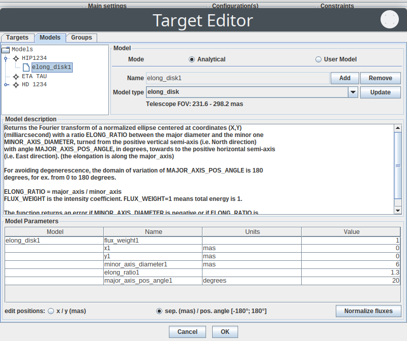
Analytical model
Each target can have its own object model composed of several elementary analytical model among:
punct-ual objectdiskwith elongated and flattened variantscirclei.e. unresolved ringringwith elongated and flattened variantsgaussiandistribution with elongated and flattened variantslimbdarkened disk
[!NOTE] The supported model list is subject to change and will evolve in the future.
On the first screen shot, only science targets and their models are present; on the second screen shot, science, calibrator targets and their models are present.
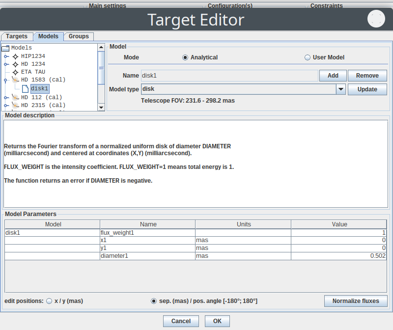
To add a new elementary model, choose first its model type and then click on the Add button.
To remove an elementary model, select first a model in the tree view and then click on the Remove button.
Of course, you can convert any elementary model to another type: select first a model in the tree view, choose the new model type and click on the Update button. Please check then parameter values and correct them as wanted.
The Telescope FOV indicates the overall field of view (telescope + spatial filter in the recombiner) that may impact the analytical model if any distance (separation, width ...) is larger than 20% of the FOV, then a warning is displayed indicating the problem.
The Model description area gives you a description of the current elementary model and its parameters. The Model Parameters table let you edit each parameter of analytical models.
When several models are defined for a target, the first model is always centered (x = y = 0 and fixed). Positions of other models can be edited using carthesian coordinates (x / y) or polar coordinates rho and theta (respectively separation and position angle following the astronomical convention from north through east) according to edit positions choice.
The Normalize fluxes button corrects values of the flux_weight parameter to have a total flux equal to 1.0.
[!NOTE] The type of coordinates (carthesian or polar) can be defined in the Preferences Window.
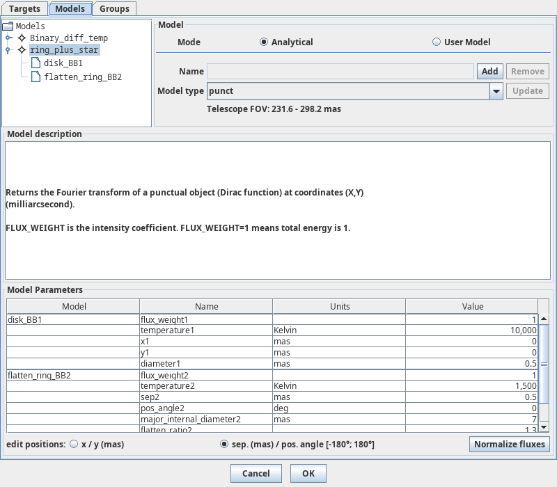
Analytical model with black-body temperature
Additionnally one can use elementary analytical model that include a black-body temperature.
disk_BBuniform disk with elongated and flattened variantsring_BBuniform ring with elongated and flattened variantsgaussian_BBgaussian function with elongated and flattened variants
[!NOTE] Models with a black-body temperature cannot be associated with grey ones. Statistics on fLux ratios per component are displayed in the Status Indicator (log) to determine how components contribute to the total flux (hence visibility).
On the following screen shot, the model is made of a resolved star (disk_BB) and a ring (ring_BB) with different temperatures and emitting surfaces:
When several (N) models with a black-body temperature are specified the resulting complex visibility is computed as:
$V_{tot}(u,v,\lambda) = \frac{\sum_i^N S_i B(\lambda, T _i) V_i(u,v)}{\sum_i^N S_i B(\lambda, T _i)}$
where $V_i(u,v)$ is the visibility of the ith component;
and the flux emitted by each component corresponds to the Planck black-body function :
$B(\lambda, T) = \frac{2hc^2}{\lambda^5} \frac{1}{(\exp^{\frac{hc}{k\lambda T}} -1)}$
$S_i$ represents the solid angle of the component.
[!IMPORTANT] For the noise computation, in the absence of distance information, it is the magnitude of the object entered by the user in
Targetstab (or retrieved via SIMBAD) that is taken into account and not the black-body flux.
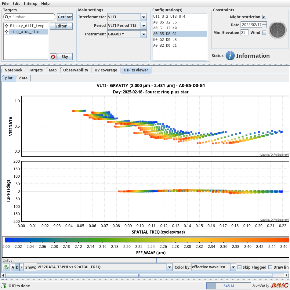
With the previous black-body model, the OIFits viewer shows the squared visibility illustrating the chromatic effect (comma shape):
User-defined model
Each target can have an user-defined model using one FITS image (monochromatic model) or cube (polychromatic model) representing the object flux over the sky (i.e. X and Y axes corresponds respectively to RA and DEC coordinates) optionally per spectral channel for Fits cubes.
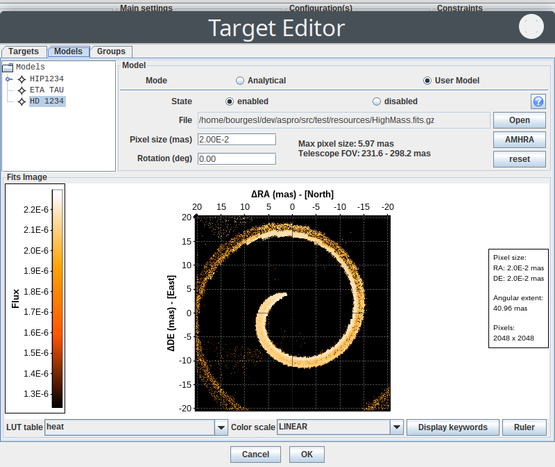
To add or change an user model, click on the Open button and choose your FITS image or cube file (fits or fits.gz files are both supported).
The image extent is displayed (too large extent will generate a warning and the image will not be displayed).
One can adjust the image extent using the Pixel size field and rotate the image using the Rotation field. This permits to "fit" any image, whatever its FITS header values, in the interferometer FOV. Of course you have to know what you do!
The Telescope FOV indicates the overall field of view (telescope + spatial filter in the recombiner) that impacts model images if their extent is larger than 20% of the FOV (see the apodization step below).
Click on the AMHRA button to open the AMHRA service that provides several polychromatic science models as FITS image cubes that can be sent back to ASPRO2 using the SAMP interoperability ('image.load.fits' message).
[!NOTE] Use the image browser widget to see all polychromatic images (Fits cube only):
When your FITS image (or cube) is loaded (only the first image / cube present in the FITS file), several image processing tasks are performed to obtain a linear-flux image prepared for Fourier transform computations:
- compute its dynamic range
- ignore negative values (set to 0.0)
- perform image apodization (if necessary) given the telescope diameter and instrumental minimum or model image wavelength by multiplying the image with a gaussian profile whose $FWHM \approx (lambda / diameter)$. Typically the telescope's PSF is 60 mas for a VLTI/UT. So if the object is very extended, ASPRO2 will only retain data within the telescope's PSF (smaller extent).
- compute the total flux $Fi$ = sum(image) to normalize the image by 1.0 / Fi i.e. sum(normalized image) = 1.0
- ignore flux values lower than an adaptive threshold [*] (i.e. set such values to 0.0) to ensure the error on visibility amplitude is lower than 1 thousandth
- extract the region of interest (centered region where flux is > 0.0 to ignore blank data pixels
- make the image square i.e. width = height = even number
[!NOTE]
- To preserve the model's integrity, rotation and scaling are performed on the visibilities only.
- The FITS image (or cube) flux unit is meaningless to ASPRO 2: the flux of the object (hence, the S/N of the computed visibilities) is always derived from the magnitude in the observation band given in the Target Editor and scaled by (Fi / Fm) for Fits cubes where Fm is the integrated flux(Fi) over the band / band width
The 5th task is only performed when the Fast mode (optimize the input image) is enabled in the Preferences Window: it consists in discarding useless data to have accurate but
faster response time when computing optimized Fast (UV plane) or direct Fourier transform (simulated OIFits data).
If your image was successfully loaded and coordinate increments are valid, the prepared image is displayed on the zoomable image preview using given LUT table and Color scale:
- on the left side, the color scale represents the normalized flux.
- on the right side, the pixel size (mas) and the angular extent are displayed. For Fits cubes, the corresponding image index and its wavelength are displayed too.
[!NOTE] As useless data pixels are discarded, the image preview displays the prepared image having useful flux data that ASPRO 2 will use in Fourier transforms. To reduce computation time, use small image sizes; moreover, zero padding in the FITS image is useless or counter productive as ASPRO 2 always performs its image processing.
Use the State field to enable or disable an user-defined model.
Actually the user-defined model may be automatically disabled if ASPRO 2 can not load its file (moved or deleted) or if coordinate increments are invalid for the selected configuration (UV Max and instrument minimal wavelength); so it is better to keep FITS image files in a folder dedicated to ASPRO 2 observations on your file system (archive).
Moreover, ASPRO 2 does not embed FITS files in its own Aspro Observation file format for the moment, but certainly in future releases. This means that such observation files can still be exchanged between colleagues but user-defined models will then be disabled. To enable them again, you must send FITS image files to your colleague and he must use either the
Open button action to open the FITS image files (placed to another location on his file system) or use the State field to enable them (same file location).
[!NOTE] ASPRO 2 computes FITS checksum to ensure file integrity and detect if an used user-defined model has changed. In such case, this model will be disabled and ASPRO 2 encourages you to check your FITS image by opening the
Target editor.
Following FITS image keywords are interpreted by ASPRO 2:
SIMPLE  =                    T / Fits standard
BITPIX  =                  -32 / Bits per pixel                                Float (REAL*4) but any data type is supported
NAXIS   =                    3 / Number of axes                                2 or 3 respectively for FITS image/cube
NAXIS1  =                  512 / Axis length                                   RA  / column
NAXIS2  =                  512 / Axis length                                   DE / row
[NAXIS3 =                    7 / Axis length                                   Optional Wavelength axis]
EXTEND  =                    T / File may contain extensions
[...]
CRPIX1  =                 256. / Reference pixel
CRVAL1  =                   0. / Coordinate at reference pixel
CDELT1  =             -1.2E-10 / Coord. incr. per pixel (original value)       rad / pixel (RA / column)
[CUNIT1 =              'RAD'   / Units along axis                              Optional axis units (rad, deg, arcmin, arcsec)]
CRPIX2  =                 256. / Reference pixel
CRVAL2  =                   0. / Coordinate at reference pixel
CDELT2  =              1.2E-10 / Coord. incr. per pixel (original value)       rad / pixel (DE / row)
[CUNIT2 =              'RAD'   / Units along axis                              Optional axis units (rad, deg, arcmin, arcsec)]
[CRPIX3 =                   1. / Reference pixel
CDELT3 =              4.75E-02 / Coord. incr. per pixel (original value)       (Wavelength increment / image)
CRVAL3 =              1.528550 / Coordinate at reference pixel                 Wavelength reference
CUNIT3 =              'MICRON' / Units along axis                              Optional axis units (meter, micron, nanometer, hertz)]
[...]
[!NOTE]
- NAXIS1 and NAXIS2 are not expected to be even number or power of two nor equals; any axis length > 1 is supported.
- Coordinate increments (RA / DEC) are mandatory and expected in DEGREES if no given unit (CUNIT keywords). Use the
ScaleandRotationfields to adjust the Coordinate increments (RA / DEC) and apply any rotation to the user model.- To get the description of the current FITS file, you can click on the
Infobutton.
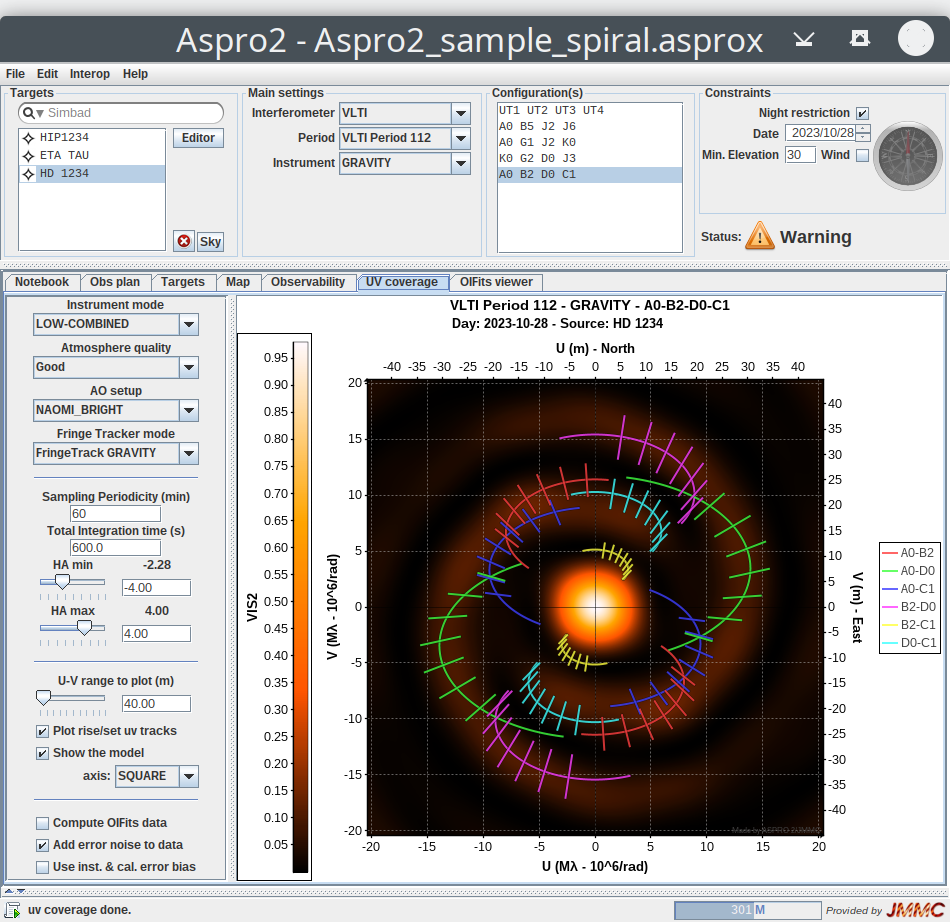
For example, the following screen shot shows the UV coverage plot of the previous spiral user-defined model:
Polychromatic User-defined model
How to use polychromatic image models to estimate flux and visibility values at each detector channel defined by EFF_WAVE (central wavelength) and EFF_BAND (channel width) arrays in the OIFITS standard.
The model gives a list of images with attributes:
- image central wavelength and the wavelength increment gives the lower and upper wavelength values i.e. the image bandwidth
- total flux $F$ (any unit) from the loaded and processed image
- normalized image data $IN$ i.e. $sum(IN) = 1$
- then the linear image data is $I = F * IN$
Given an instrument and a specific instrumental mode, for each channel ($\lambda_i$, $d\lambda_i$):
- $Vis(\lambda_i) = \frac{FT [ Model(\lambda_i) ]}{Flux [ Model(\lambda_i) ]}$
If the model is mono-chromatic or a single model image A corresponds to the detector channel at lambda_i (channel and image bandwidth overlap OR the closest image if interpolation disabled or extrapolation enabled), then it simplifies to:
- $I(\lambda_i) = I_A = F_A * IN_A$
- $F(\lambda_i) = F_A$
- $Vis(\lambda_i) = \frac{FT [ I_A ]}{F_A} = FT [ IN_A ]$
If Interpolation is enabled and 2 model images A and B exist where $\lambda_A <= \lambda_i <= \lambda_B$, then a linear interpolation on the image flux can be performed:
-
$\alpha = \frac{ \lambda_B - \lambda_i }{ \lambda_B - \lambda_A }$
-
$I(\lambda_i) = \alpha * I_A + (1 - \alpha) * I_B $
-
$I(\lambda_i) = \alpha * F_A * IN_A + (1 - \alpha) * F_B * IN_B $
-
$F(\lambda_i) = \alpha * F_A + (1 - \alpha) * F_B $
-
$Vis(\lambda_i) = \frac{ FT [ I(\lambda_i) ]}{ Flux(\lambda_i)}$
-
$Vis(\lambda_i) = \frac{ \alpha * F_A * FT [ IN_A ] + (1 - \alpha) * F_B * FT [ IN_B ] } { \alpha * F_A + (1 - \alpha) * F_B } $
With Interpolation, the visibility is a linear combination of Fourier transforms of the A and B normalized images.
For Fits cubes, OI_FLUX's FLUXDATA / FLUXERR columns give the object flux and error (from the object magnitude) scaled by $\frac{Fi}{Fm}$ where $Fm$ is the integrated flux $Fi$ over the band / band width: $$Fm = \frac{ \int_{\lambda_{Bmin}}^{\lambda_{Bmax}} Fi.\delta\lambda }{\lambda_{Bmax} - \lambda_{Bmin}}$$
[!NOTE]
- Extrapolation allows to use the first and last image of the polychromatic image model to compute visibilities for detector wavelengths smaller and larger than provided by the model.
- Interpolation and Extrapolation on user-models can be enabled / disabled in the Preferences Window.
Groups Tabbed Pane
The Groups panel allows you to Drag & Drop targets to define groups and associations, in particular to associate ancillary stars to your SCIENCE or CALIBRATOR objects using the predefined groups:
- AO (Adaptive Optics),
- FT (Fringe Tracker),
- Guide stars.
In the following screenshot, 'Sirius B' uses the 'Sirius A' star for the AO sub-system:
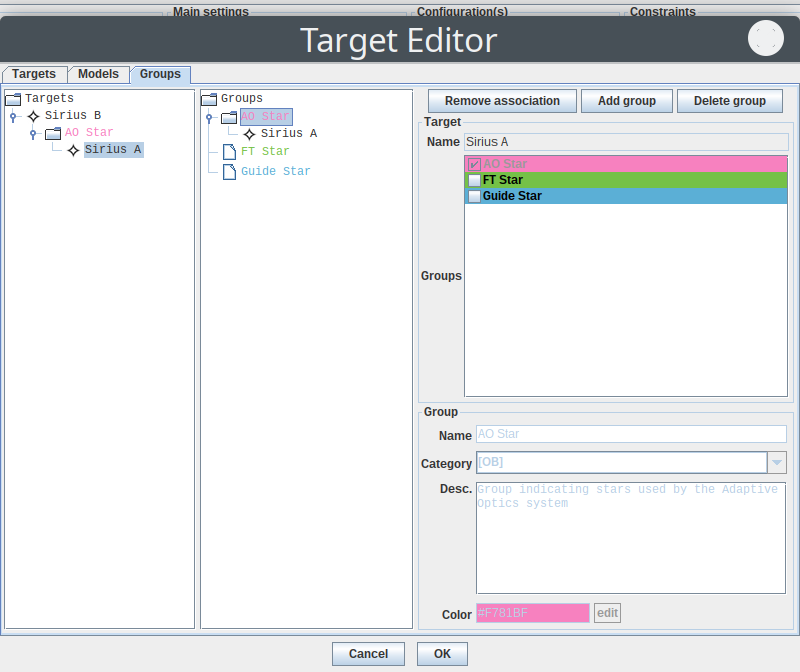
On the left side, all SCIENCE / CALIBRATOR targets are shown with their associated stars. On the middle tree panel, target Groups are shown with their corresponding stars; stars can belong to multiple groups. On the right side, target groups are displayed for the selected target (see checked boxes) and the group information is displayed for the selected group.
To mark a target as AO / FT / Guide stars, select it on the left side and either click on the corresponding Group(s) (AO star, FT star, Guide star) or use Drag & Drop to the appropriate Group in the tree on the middle (Target groups with their associated targets).
To associate an AO / FT / Guide star to your SCIENCE / CALIBRATOR target(s), use Drag & Drop from the selected ancillary star in the appropriate AO / FT / Guide Star Group to the corresponding SCIENCE / CALIBRATOR target. To discard such association between targets, select the ancillary star and use the Remove association button.
To create user-defined groups, use the Add group button and edit its name, description and color. Only empty user-defined groups can be removed using the Delete group button.
[!NOTE] Target groups (AO / FT) are used by the noise modelling and A2P2 interoperability. See ASPRO2 - How to prepare VLTI's GRAVITY or MATISSE observations with new GPAO ?
Preferences
This window let you define several settings that are stored on your machine and will be loaded at application start up.
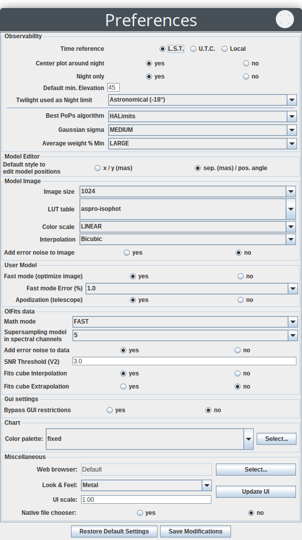
Preferences are grouped by feature:
- Observability
- Model editor
- Model Image
- User Model
- OIFits data
- Miscellaneous: it gathers several preferences related to the default web browser, Look and Feel and GUI up-scaling for Hi-DPI screens (retina or 4K); please test your UI scale factor using the
Update UIbutton but it is recommended to restart the application once the proper value is set.
Use the Restore Default settings button to reset your preferences to default values and Save Modifications to make you changes persistent; otherwise, your settings will be used until you close ASPRO 2.
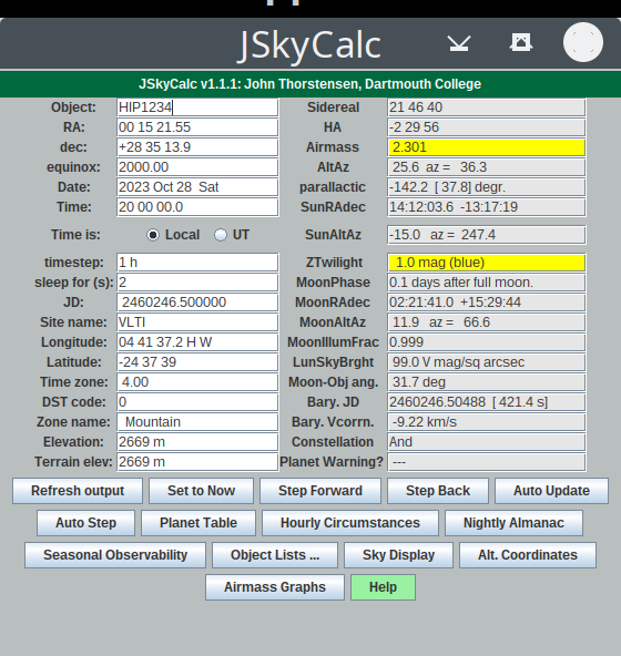
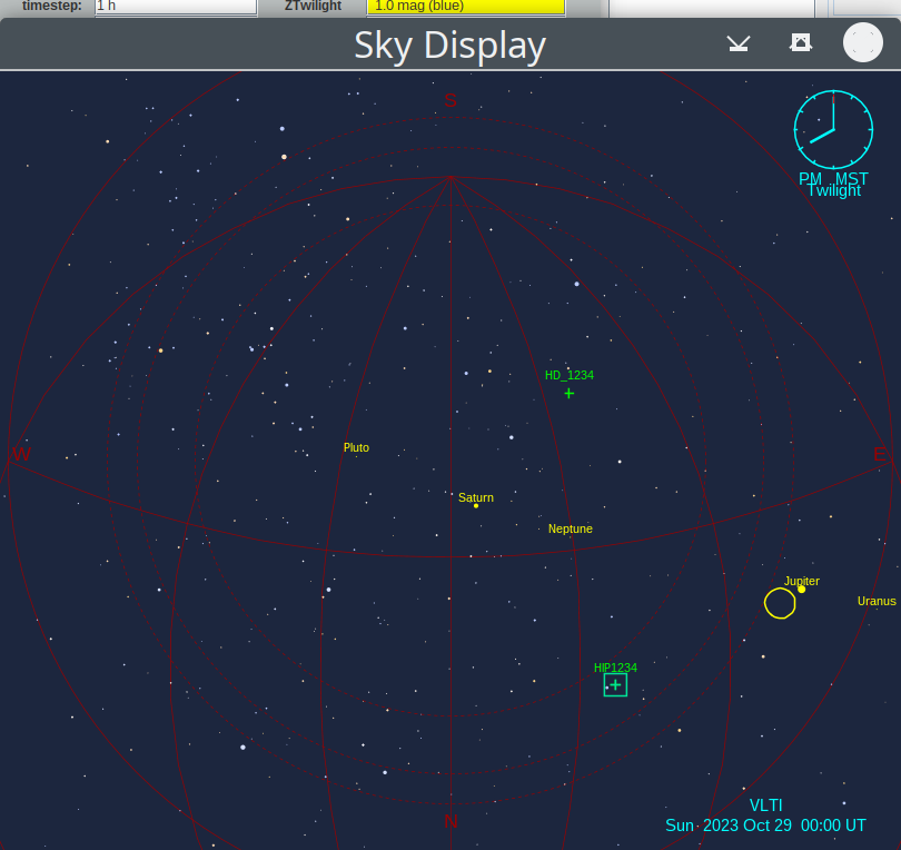
JSkyCalc tool
The JSkyCalc tool made by J. R. Thorstensen, Dartmouth College has one main window with all lot of buttons which shows / hides a pop up window per feature:
- live sky display showing moon, planets, your targets indicated by a cross symbol and its name
- airmass plot(s) for the selected object or all targets
- hourly circumstances, nightly almanac, seasonal observability, planet table ...
[!NOTE]
- Click on the
skybutton on the ASPRO 2 main panel to synchronize your observation (observatory location, target list, date, and time set to 20:00 Local time)- All JSkyCalc windows are synchronized i.e. all plots / windows are refreshed if you add / remove a target or modify the current date / time.
- Closing the main window will close also all opened pop up windows
Click on the Help button to open the JSkyCalc documentation page.
Interoperability
JMMC applications are able to communicate with other VO tools (VO stands for virtual observatory) using SAMP (Simple Applications Messaging Protocol) messaging protocol (see IVOA SAMP for more information).
Here are JMMC applications supporting the SAMP messaging protocol:
- AppLauncher ensures VO interoperability by managing the SAMP hub and automatically start VO tools
- ASPRO 2 interacts with JMMC SearchCal, LITpro, OIFits Explorer / OImaging (custom message types) and accepts incoming messages in FITS image or VOTable format (target list) from any VO tool (Simbad, ViZier, Topcat ...)
- SearchCal interacts with ASPRO 2 and any VO application supporting VOTable (Topcat ...)
- LITpro accepts incoming messages from ASPRO 2 and exports data tables to Topcat
- AMHRA service exports FITS image cubes to ASPRO2 or OImaging
The following page gives you the official list of VO applications supporting SAMP messaging protocol: IVOA SAMP Software
General description: The communication architecture is the following: all tools communicate with a central "Hub" process, so a hub must be running in order for the messaging to operate. If a hub is running when a JMMC application starts, or if one starts up while any JMMC application is in operation, it will connect to it automatically. A hub can be started from within any JMMC application if needed. Other tools will have their own policies for connecting to the hub, but in general it is a good idea to start a hub first before starting up the tools which you want to talk to it.
This communication has two aspects to it: on the one hand an application can send messages to other applications which causes them to do things, and on the other hand an application can receive and act on such messages sent by other applications.
SAMP in JMMC applications
When a JMMC application starts, it will try to connect to an existing hub or start a new internal hub.
The running hub is indicated by the  system tray icon that provides following actions:
- use
Show Hub windowto see registered applications - use
Stop Hubto stop the hub and disable communications between applications (not recommended)
Here is a screen shot of the hub status window:
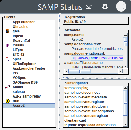
Anyway when the JMMC application is started, it will be ready to communicate with other JMMC (and VO) applications.
JMMC applications have an Interop menu containing common actions followed by specific actions to send messages to other applications:
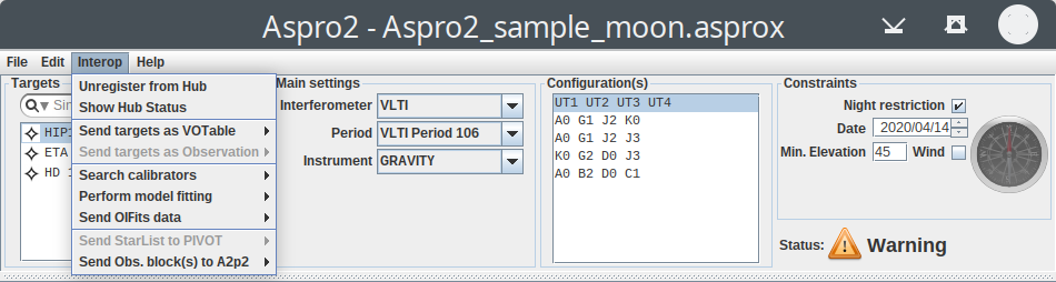
Common actions are:
Register With Hubaction connects this application to the running hub; if no hub is running, a confirmation dialog asks you if you want to start an internal hub and connect to it.Unregister from Hubaction disconnects this application from the hub; other applications can no more communicate with this applicationShow Hub Statusaction opens the hub window to see registered applications
[!NOTE]
- If you close the JMMC application which started the hub, other applications will be disconnected and no hub will be running any more.
- In this case, you should use the
Register With Hubaction to start another hub and other JMMC applications will reconnect to it automatically.
ASPRO 2 / SearchCal
How to find calibrators easily using SearchCal from ASPRO 2 ?
SearchCal is a tool developed by the JMMC Working Group "catalogue of calibration sources" to assist the astronomers in this calibrator selection process for long baseline interferometric observations.
[!NOTE]
- As SearchCal uses the JMMC server to operate, an internet connection is required.
- SearchCal 4.3+ is required to support interoperability with ASPRO 2.
Here is a step by step tutorial:
- Start the SearchCal application (or it is already running) to be able to communicate with it: SearchCal
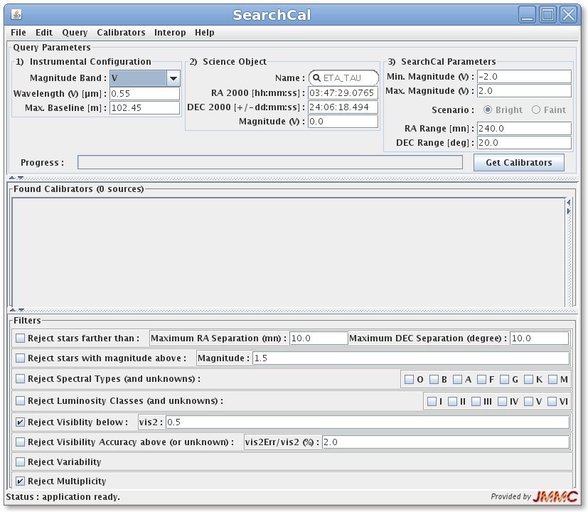
- In ASPRO 2, select your science target in the target list and use the
Search calibratorsaction in theInteropmenu to let ASPRO 2 send a message to SearchCal with your target information (coordinates, magnitudes), the instrument band and other parameters (maximum baseline length):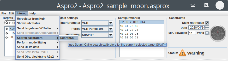
- SearchCal interprets the ASPRO 2 message, updates its graphical user interface and sends the query immediately (please wait). When calibrators are found, they are filtered and displayed:
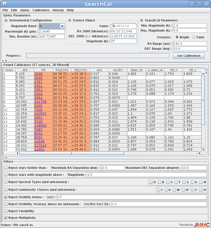
- Select the calibrators you want or all displayed calibrators (i.e. filtered) will be sent to ASPRO 2.
- Use the
Send calibrators toaction in theInterop Menuto let SearchCal send these calibrators to ASPRO 2: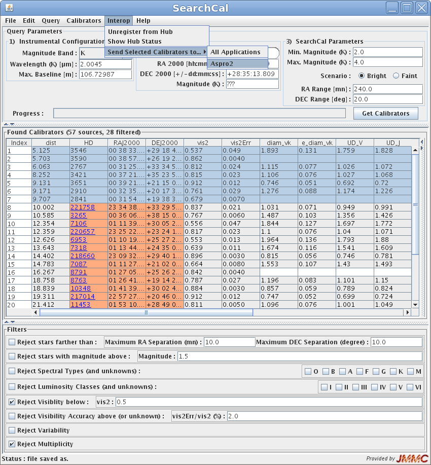
- ASPRO 2 processes the SearchCal message and displays an operation summary:
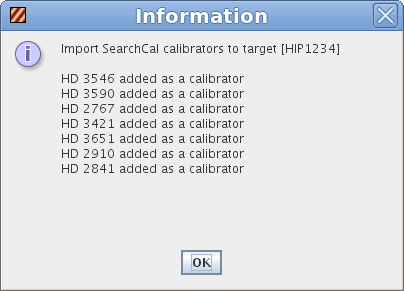
- That's all: ASPRO 2 has updated the target list with SearchCal calibrators, created an uniform disk model for every calibrator target using the SearchCal diameter corresponding to the instrument band (UD_ fields) and the graphical user interface is updated:
- Observability plot:
calibrators are represented in blue and are located below their related science target:
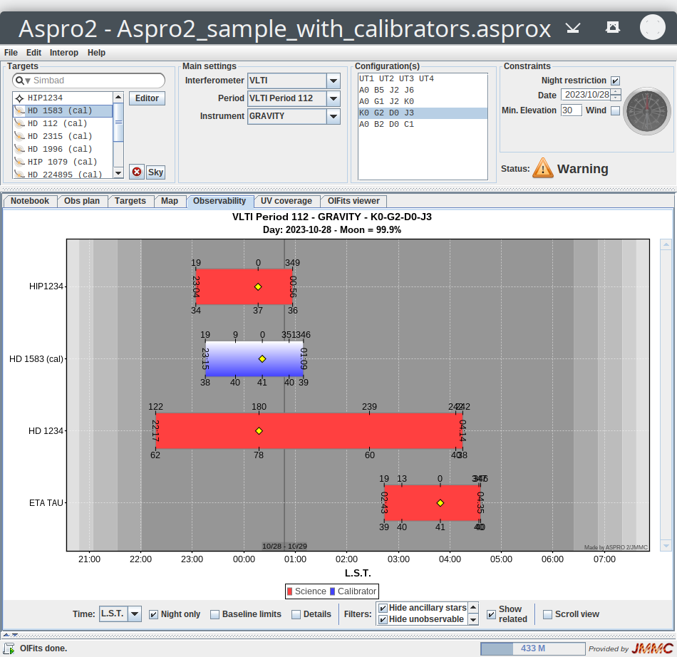
- UV Coverage plot for a SearchCal calibrator target:
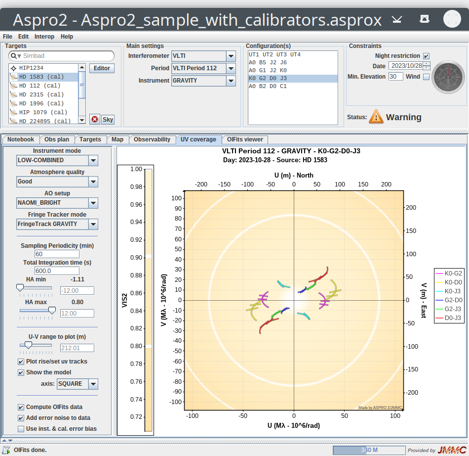
- Target editor with calibrators:
[!NOTE]
- If you choose another instrument or instrument mode (i.e. instrument band), SearchCal calibrators may become inappropriate. Look at the UV Coverage plot to verify that one calibrator target is still a "good" calibrator for your observation.
- Moreover, you can still use the Calibrator Information which contains uniform disk diameters (per band) to get the correct diameter value and use it to set the diameter value of the disk model associated to one calibrator target.
ASPRO 2 / LITpro
How to prepare easily your model fitting using LITpro from ASPRO 2 ?
LITpro is a model fitting software, developed and maintained by one JMMC working group ( CRAL, LAOG and FIZEAU ).
[!NOTE]
- As LITpro uses the JMMC server to operate, an internet connection is required.
- LITpro 1.0.7+ is required to support interoperability with ASPRO 2.
Here is a step by step tutorial:
- Start the LITpro application (or it is already running) to be able to communicate with it: LITpro
- In ASPRO 2, select your target in the target list and use the
Perform model fittingaction in theInteropmenu to let ASPRO 2 send a message to LITpro with your simulated OIFits file and target information (with object model) as shown on the UV Coverage plot: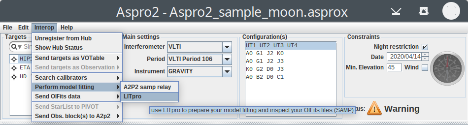
- LITpro interprets the ASPRO 2 message, loads the OIFits file and displays the OIFits validation summary:
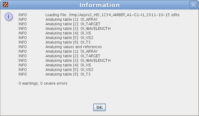
- That's all: LITpro has now updated the graphical interface with the new created settings including the OIFits file and the target with its object model:
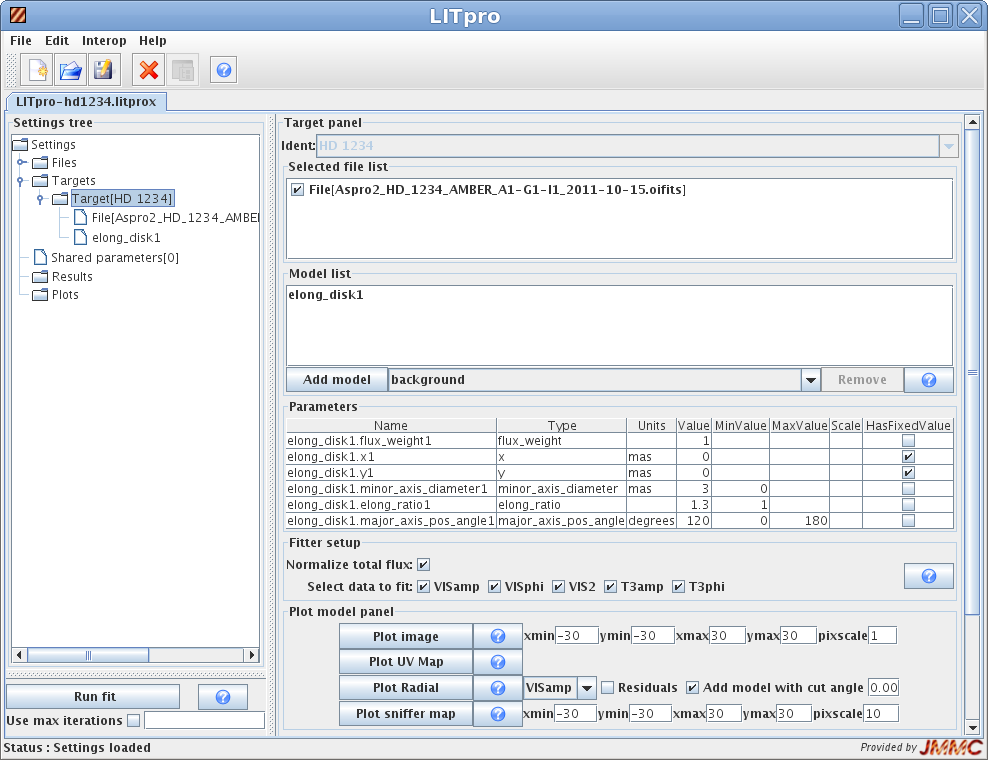
- LITpro shows the content summary of OIFits files:
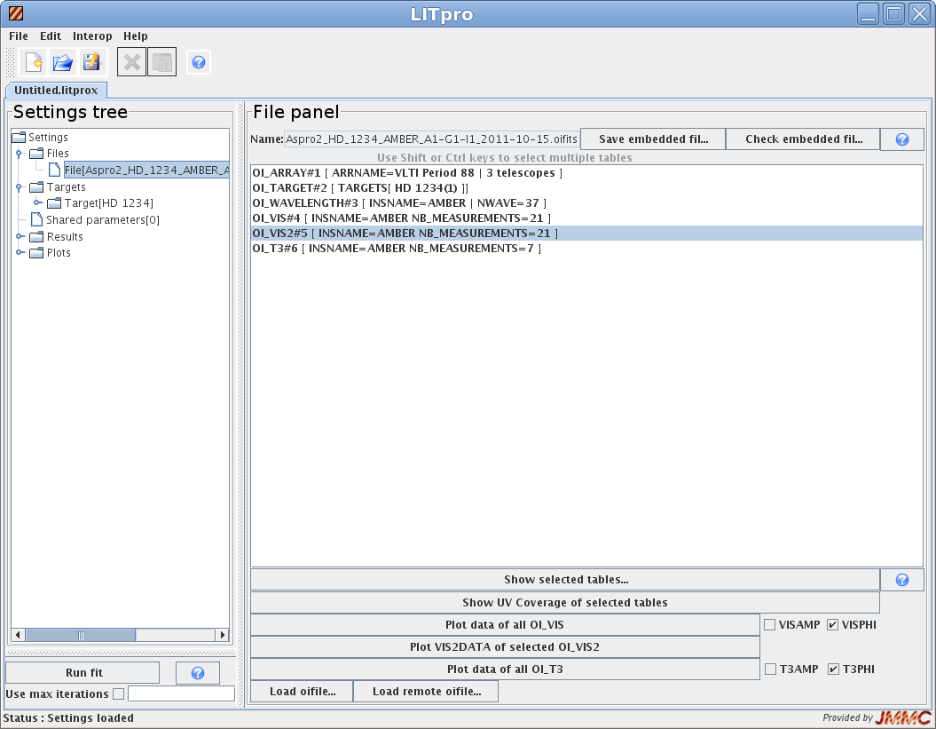
- LITpro can also plot any data table (OI_VIS, OI_VIS2, OI_T3):
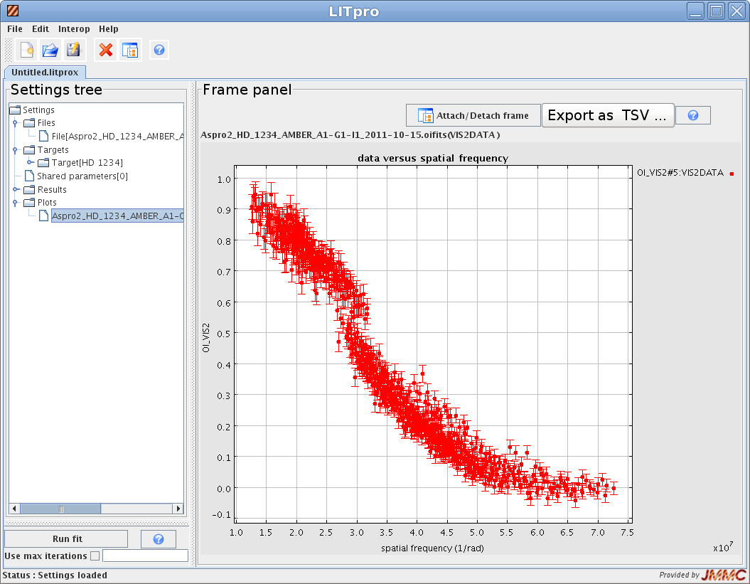
ASPRO 2 / OIFits Explorer
Using the Send OIFits data action in the Interop menu, you can send your simulated OIFits file to the OIFitsExplorer / OImaging or any other VO tools supporting FITS files.
It can be very helpful in several use cases:
- combine simulated data (ASPRO 2) with observed data for your target to adjust your observation proposal (hour angle, UV coverage)
- combine simulated data (ASPRO 2) from different interferometer or instruments (extended multi configuration)
- evaluate the image reconstruction of simulated OIFITS data with OImaging
ASPRO 2 / A2P2
Using the Send Obs. block(s) to A2p2 action in the Interop menu, you can send an Observing Block of the selected target to A2P2, the
ASPRO2 bridge to ESO P2 or CHARA backends.
See the A2P2 project on github: ASPRO2 / A2P2 Tutorial
ASPRO 2 - Export targets to VO Tools
Using the Export targets to VOTable action in the Interop menu, you can send your target list to any other VO tools supporting VOTable files (another ASPRO2 instance, Topcat or Aladin for finding charts).
ASPRO 2 - Import targets from VO Tools
ASPRO 2 supports the standard 'table.load.votable' SAMP message to import a target list from any VO Tool (Topcat, Vizier ...) using the VOTable format (version 1.1 and 1.2) conforming to the following rules:
- Single RESOURCE and TABLE containing target data using TABLEDATA serialization only
- Coordinate system (COOSYS) is eq_FK5 / J2000 (STC not supported)
- Specific ASPRO 2 parameters can define also its configuration (interferometer, instrument, baseline ...) for advanced use cases: contact the user support team if you are interested
- Data columns are interpreted using UCD i.e. Uniform Content Descriptors (version 1.0 and 1.1) and their units
Supported data columns are listed in the following table:
| Name | Description | Data type | UCD 1.0 | UCD 1.1 | Supported Units |
| NAME | Target name (identifier) | char | META.MAIN | meta.id;meta.main | |
| RA | Right ascension - J2000 | char | POS_EQ_RA_MAIN | pos.eq.ra;meta.main | 'h:m:s' or 'hms' or 'deg' |
| DEC | Declination - J2000 | char | POS_EQ_DEC_MAIN | pos.eq.ra;meta.main | 'd:m:s' or 'dms' or 'deg' |
| RV | Radial velocity | double | VELOC_HC | spect.dopplerVeloc.opt | 'km.s-1' or 'km/s' |
| PMRA | Proper motion in RA | double | POS_EQ_PMRA | pos.pm;pos.eq.ra | 'mas.yr-1' or mas/yr |
| PMDEC | Proper motion in DEC | double | POS_EQ_PMDEC | pos.pm;pos.eq.dec | 'mas.yr-1' or mas/yr |
| PLX | Parallax | double | POS_PARLX_TRIG | pos.parallax.trig | mas |
| e_PLX | Parallax error | double | POS_PARLX_TRIG_ERROR | stat.error;pos.parallax.trig | mas |
| HD | HD identifier (H. Draper: III/135A) | char | META.ID | meta.id | |
| HIP | HIP identifier (Hipparcos catalogue: I/239) | char | META.ID | meta.id | |
| 2MASS | 2MASS identifier (2Micron All-Sky Survey: II/246) | char | META.ID | meta.id | |
| OTYPES | Object type(s) | char | src.class | ||
| SP_TYPES | MK spectral type(s) | char | SPECT_TYPE_MK | src.spType | |
| FLUX_V | Magnitude V | double | PHOT_JHN_V | phot.mag;em.opt.V | mag |
| FLUX_I | Magnitude I | double | PHOT_JHN_I | phot.mag;em.opt.I | mag |
| FLUX_J | Magnitude J | double | PHOT_JHN_J | phot.mag;em.IR.J | mag |
| FLUX_H | Magnitude H | double | PHOT_JHN_H | phot.mag;em.IR.H | mag |
| FLUX_K | Magnitude K | double | PHOT_JHN_K | phot.mag;em.IR.K | mag |
| FLUX_N | Magnitude N | double | PHOT_JHN_N | phot.mag;em.IR.8-15um | mag |
[!NOTE] Only Name and coordinates (RA/DEC) are mandatory. Supported identifiers must use correct column names (HD, HIP, 2MASS).
Here is a sample VOTable file describing all possible parameters and columns: Aspro2_samp_load_votable.xml: Aspro2 Sample Target list (VOTable)
ASPRO 2 - Import FITS image from VO Tools
ASPRO 2 supports the standard 'image.load.fits' SAMP message to import one FITS image or cube from any VO Tool (AMHRA, OImaging, LITpro, DS9 ...).
As described in the User Model section, the FITS image or cube must provide mandatory keywords (increments, units...) to be compatible in terms of spatial and spectral resolution with the observation setup (instrument, baselines).
ASPRO 2 - Command Line Interface
ASPRO2 provides a simple command line interface to compute interferometric observables from one input OIFits file and a user model image (FITS cube) and produce another OIFits file containing computed observables from the model at the spatial frequencies (UV plan) given by the input OIFits file (typically an observation data file).
If the given user model image's wavelength range is smaller than the instrumental wavelength range (OI_WAVELENGTH effwave range), then observables can not be computed and set to NaN (extrapolation disabled by default). As it does not perform the noise modelling, errors are left undefined (NaN), but chi2 are computed too.
Command line syntax
The following command starts ASPRO2 in shell mode (no GUI) with the argument -process and its mandatory arguments -input, -output and -image to give full paths to the OIFits files and the FITS image file.
java -jar Aspro2-Version.jar -process -input <input OIFits file> -image <fits file> -output <output OIFits file>
Here is a sample script showing several processing cases with optional arguments: test-process.sh
Command line arguments
The following command gives the full list of arguments (default values are given within brackets):
java -jar Aspro2-Version.jar -help
---------------------------------- Arguments help ------------------------------
| Key          Value           Description                                     |
|------------------------------------------------------------------------------|
| [-h]                         Show the options help                           |
| [-h|-help]                   Show arguments help                             |
| [-loggui]                    Show the logging tool                           |
| [-v]         [0|1|2|3|4|5]   Define console logging level                    |
| [-version]                   Show application name and version               |
| [-open <file>]               Open the given file (if supported)              |
|------------------------------------------------------------------------------|
| [-process]                   process an OIFITS file and model to compute observables [SHELL]    |
| [-image]                     the input FITS model to process [SHELL]    |
| [-input]                     the input OIFITS file to process [SHELL]    |
| [-output]                    the output OIFITS file to write [SHELL]    |
| [-fast]                      [true] to ignore useless data; false to have highest precision [SHELL]    |
| [-fastError]                 optional Fast mode error in percents [0 - 10 %]; 1% by default [SHELL]    |
| [-supersampling]             supersampling per spectral channel [5] [SHELL]    |
| [-math]                      Math mode: ['FAST'] faster, 'DEFAULT' highest accuracy or 'QUICK' fastest BUT low accuracy [SHELL]    |
| [-scale]                     optional image scale (increment) expressed in milli-arcsec (mas) [SHELL]    |
| [-rotate]                    optional image rotation expressed in degrees [SHELL]    |
| [-apodize]                   [true] to perform image apodization; false to disable [SHELL]    |
| [-diameter]                  optional telescope diameter (meters) used by image apodization [SHELL]    |
| [-modelInterpol]             [true] to perform linear interpolation between FITS cube images; false to disable [SHELL]    |
| [-modelExtrapol]             true to compute spectral channels out of the FITS cube wavelength range; [false] to disable [SHELL]    |
|------------------------------------------------------------------------------|
LOG LEVELS : 0 = OFF, 1 = SEVERE, 2 = WARNING, 3 = INFO, 4 = FINE, 5 = ALL
These optional arguments correspond to ASPRO2's Preferences used by User-defined model processing (fast mode & error, supersampling, scale & rotate model image, apodization, fits cube interpolation & extrapolation).
See Polychromatic User-defined model
Support and change requests
Please do not hesitate to use the JMMC Feedback Report integrated using Help menu / Report Feedback to JMMC... action:
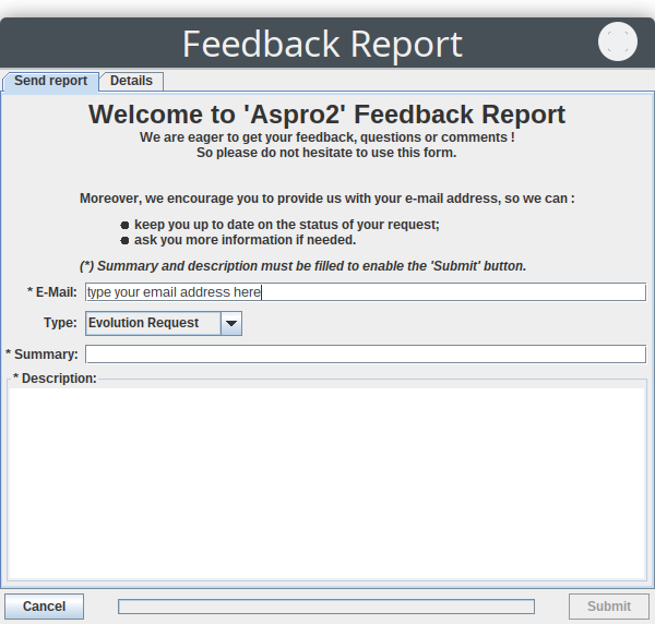
Of course, you can still contact the user support team for any bug report or change request.
[!NOTE] If an unexpected exception occurs in a JMMC application, an error message will be displayed and the JMMC Feedback Report will be opened to encourage users to submit their problems and let the JMMC technical team fix it as soon as possible
Sample files
Here are the "Guided Tour" Observation files that can be loaded in ASPRO 2 / SearchCal / LITpro for demonstration purposes:
- Aspro2_sample.asprox: Sample observation file
- Aspro2_sample_multi.asprox: Sample observation file (multi configuration)
- Aspro2_sample_with_calibrators.asprox: Sample observation file completed with SearchCal calibrators for HIP 1234
- SearchCal-hip1234.scvot: SearchCal VOTable for HIP 1234
- LITpro-hd1234.litprox: LITpro Settings for HD 1234
The following folder gives sample output files (PDF, OIFITS files): outputs